Discrete Dynamical Systems: From Theory to Real-World Impact

Dive into the world of discrete dynamical systems. Understand fundamental equations, analyze long-term behaviors, and apply your knowledge to solve real-world problems in ecology, economics, and more.

Discrete dynamical systems

Dynamic system definition

We define dynamic system as a body pertaining to a geometrical space which depends on time. This time dependence means that such a system changes as time progresses and there is a mathematical function which describes such change.

In simple words, a dynamical system refers to any system that changes through time and so, its state can be explained and observed at any particular moment or lapse in time, but this state will not be the same as time progresses. Dynamical systems can be classified as discrete and continuous dynamical systems depending on the size of the periods of time required for the system to change, or transform. We will talk about the differences of the two in the next section, for now let us put this concept into context:
Since everything in our world changes as time passes by, the idea of a dynamical system can be applied to an infinite amount of scenarios to be studied mathematically. For example: the water flowing through a river is a system in constant change. Another example is a building being built. Notice that these two cases are very different and they change in steps of time in different scales, but both of them are dynamical, they move, they change state, they are not the same as they were in an earlier stage of their history.

Discrete and continuous dynamical systems

Once we have learnt the dynamic system definition, let us have an introduction to dynamical systems continuous and discrete.

Take again the examples mentioned in the last section: the river water flowing and the construction of a building, as we all know, they are both changing but notice how they do it: the water in the river is continuously flowing through and so, every infinitesimally small moment in time, the particles of water that passed through a certain point of the length of the river are gone onto another location by the next moment; on the other hand, a building in construction will change every certain periods of time that are palpable, very definable by conditions of the system, in other words, changes in construction of that building will be noticeable by the day: workers come in the morning, work their 8-hour shifts and by the end of the day they finished a certain part of the project and so they have a recount of what was done for that day. At the end of that day the state of the building changed, but you cannot go back into minutes or seconds during the day and see palpable difference from the day before, until the project for the day has been finished, you can now say oh today this and that was done.

That is the difference between continuous and discrete dynamical systems. A continuous dynamical system, as its name mentions, changes CONTINUOUSLY, meaning that it changes by every infinitesimally small moment in time. The water at certain point in the river is gone to another location in fractions of a second, the same as our aging process that every moment in time that passes is changing progressively and there is no way to stop the process until is done.
Then, a discrete dynamical system is that system which requires of specific periods of time to produce a change, in this case, the construction of a building will have certain changes for a day, then the workers go home and the state of the building remains unchanged until they come back next day and achieve a new change. The state of the system varies by separate points of time, but in between these points there is no change.

The names of the dynamical systems then come from how time as a variable is taken on them, time is a continuous variable when studying continuous dynamical systems, while time is a discrete variable (looked as in measurable steps) when studying discrete dynamical systems. Continuous dynamical systems require differential equations for their study, and so, today we will focus on discrete dynamical systems only.

Discrete dynamical system

It is time for us to focus on the mathematics of the topic for today, and so, it is time for us to learn about the differential equation of a discrete dynamical system:

$x_{k+1} = Ax_k$
We have said already that a discrete dynamical system is a system which is changing through time and for this system, time is seen as a discrete variable, in other words, the system is changing by lapses of time, every particular lapse an specific change (not a continuum of progression). Thus, to define this mathematically, we will have to derive what is called the differential equation for the discrete dynamical system (notice differential means is changing through a variable, and for this case is through the variable of time).

And so, in order to produce the mathematical expression for discrete event dynamics systems, let us assume we have a matrix A, which is diagonalizable, and which has n linearly independent eigenvectors $v_1, v_2, ... , v_n$ and their corresponding eigenvalues $\lambda_1, \lambda_2, ... , \lambda_n$. Then we can write an initial vector $x_0$ to be:

$x_0 = c_1 v_1 + c_2v_2 + ... +c_nv_n$
And no, we perform a transformation of $x_0$ with matrix $A$.
Remember from our lesson on image and range of linear transformations, that a linear transformation is defined as: $T(x)=Ax$ where $A$ is a matrix and $x$ is a vector. Then, from our lesson on eigenvalues and eigenvectors , we learnt that multiplying $A$ by an eigenvector $x$ just rescales the vector with a corresponding scalar which is called and eigenvalue following the condition $Ax= \lambda x$. Therefore, if we say that we are to transform $x_0$ with matrix $A$, we will have that $T(x_0)=Ax_0= \lambda x_0$ (for each eigenvalue of $A$). We call the new re-scaled vector coming from this transformation $x_1$ and so, we have that is defined as:

$x_1=Ax_0=c_1Av_1 \,+ \, c_2Av_2 \, +...+ \, c_nAv_n = c_1 \lambda_1 v_1 \, + \, c_2 \lambda_2 v_2 \, +...+ \, c_n \lambda_n v_n$
Equation 3 is what we call the first transformation of the initial vector $x_0$. We could continuing transforming the initial vector with the matrix, lets say we do it a second time and we call this new resulting vector $x_2$, therefore, this second transformation would have to satisfy the condition: $x_2 = Ax_1= \lambda x_1\,$ for each corresponding eigenvalue of $A$, and would be defined as:

$x_2 = Ax_1 = c_1 \lambda_1 Av_1 \, + \, c_2 \lambda_2 Av_2 \,+...+ \, c_n \lambda_n Av_n$
$x_2 = c_1 \lambda_1 \lambda_1 v_1 \, + \, c_2 \lambda_2 \lambda_2 v_1 \, +...+ \, c_n \lambda_n \lambda_n v_n$
$x_2 = c_1 \lambda^{2}_{1} v_1 \, + \, c_2 \lambda^{2}_{2} v_2 \,+...+ \, c_n \lambda^{2}_{n} v_n$
So in the same way as the initial vector $x_0$ was transformed here a second time, we could continue transforming it as many times as we want. Each of this transformations is the way how the system described in the initial vector is evolving through time, specifically, through particular lapses of time, and each of those lapses is represented by the transformations.

In other words, if we are to transform a vector $k$ amount of times, all of these transformations will define the state of the system from the initial vector at any particular lapse after that particular transformation, in other words, the change for the system in that particular amount of time. The system will not change until another transformation is applied (so, the system is not continuously changing through every infinitely small moment of time time, is just changing through every specific lapses of time, or pieces of time, defined by the transformations.
The general formula to define the change a system went through for $k$ number of transformations is:

$x_k = c_1 \lambda^{k}_{1} v_1 \, + \, c_2 \lambda^{k}_{2} v_2 \, +...+ \, c_n \lambda^{k}_{n} v_n$
Which gives sense to equation 1: $x_{k+1} = Ax_{k}$ because all equation 1 is saying is that one more transformation ( one more than k) has been done to the system. Or in other words, after passing through k transformations, the system has gone through another one because another defined lapse of time has passed and the state of the system is now defined by equation 1: $x_{k+1}$.

Equation 5 is very useful because it will allow you to see the behaviour or a system, and the changes of state that it goes through discrete pieces of time. Such equation is then useful not only for mathematical studies but also for physics, biology and chemistry (actually, this is good for any branch of science, since it allows you to study the changes in behaviour or stage evolution of anything, object or body, that changes through time, which is EVERYTHING!).

Let us work through an example exercise where we will be finding the general solution to the discrete dynamical system as defined:

Example 1

Let A be a 3x3 matrix with eigenvalues 3, 2 and 1/2 , and the corresponding eigenvectors: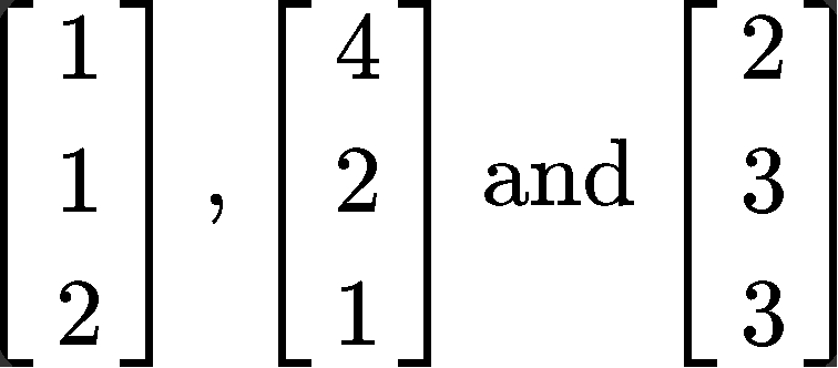


Find the general solution of the equation $x_{k+1}=Ax_k$ if the initial vector $x_0$ is defined as:


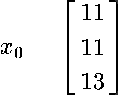
Since we have 3 eigenvalues and their corresponding 3 eigenvectors, we can automatically rewrite equation 5 for the general solution to this problem:

$x_k=c_1 \lambda^{k}_{1}v_1 \, + \, c_2 \lambda^{k}_{2} v_2 \, + \, c_3 \lambda^{k}_{3} v3$

But a problem arises, what are the values of $c_1, c_2, c_3$? In order to obtain those constant values we have to write the initial vector expression following equation 2:


Notice that we have transformed the expression for the initial vector $x_0$ into a matrix equation that we can use to solve for the values of $c_1, c_2, c_3$. Thus, we rewrite this matrix equation as an augmented matrix and row-reduce it into its reduced echelon form in order to obtain the constant values:







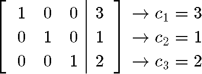
And so the values of the constants are: $c_1=3, c_2=1, c_3=2$ . Using this we can write our final answer:

Example 2

Explain the long term behaviour ($k \;$→$\; \infty$)of the equation $x_{k+1}=Ax_k$, where the matrix $A$ is defined as:


And the initial vector contains the two components $c_1 > 0, c_2 > 0$, and is defined as:


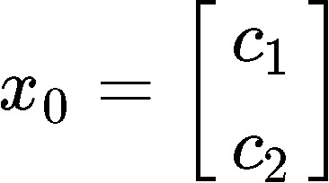
Since we want to explain long term behaviour, then it means we want to find the general solution of the way the system is changing through time, therefore, we are being asked to find the expression for $x_k$ as shown in equation 5. The problem here is that we are not given neither the eigenvalues or eigenvectors of the provided matrix $A$, therefore, our first step to work through this problem in to find them:
Using the characteristic equation $det (A-I\lambda )=0$ we solve for the eigenvalues:



So the eigenvalues are: $\lambda 1 = 1.32 \;$and$\; \lambda 2 = 1.1$
In order to find the eigenvectors associated with it, we use the relationship $(A-I\lambda )v=0$ where $v$ is the eigenvalue associated to the eigenvector used. And so, for $\lambda 1 = 1.32$ we have:



With this, we can form an augmented matrix and solve for the components of the eigenvector associated to the eigenvalue $\lambda 1=1.32$.



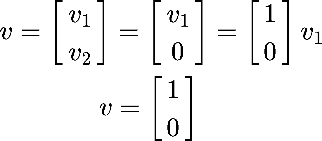
And so, we see that $v_1$ is a free variable (that we will set equal to 1 ) and $\, v_2=0$, then our eigenvector for this case is:


Now for$\lambda_2$ =1.1 we have:


And the augmented matrix to solve for the components of the eigenvector associated to the eigenvalue $\lambda_2$ =1.1


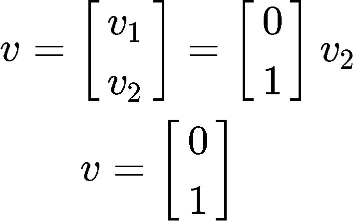
And so, we see that $v_1=0 \,$ and $\, v_2$ is a free variable that we will set equal to 1, then our eigenvector for this case is:


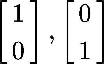
Therefore, for this problem we have that the eigenvalues are: $\lambda_1=1.32 \,$ and $\, \lambda_2=1.1 \,$ and the corresponding eigenvectors are:


Having this, we can finally write the expression for $x_k = c_1 \lambda^{k}_{1} v_1 \, + \, c_2 \lambda^{k}_{2} v_2$


With the expression found in equation 22 we can finally talk about the long term behaviour of the system as $k \;$→$\; \infty$. Look what happens to equation 22 when $k$ goes to infinity:


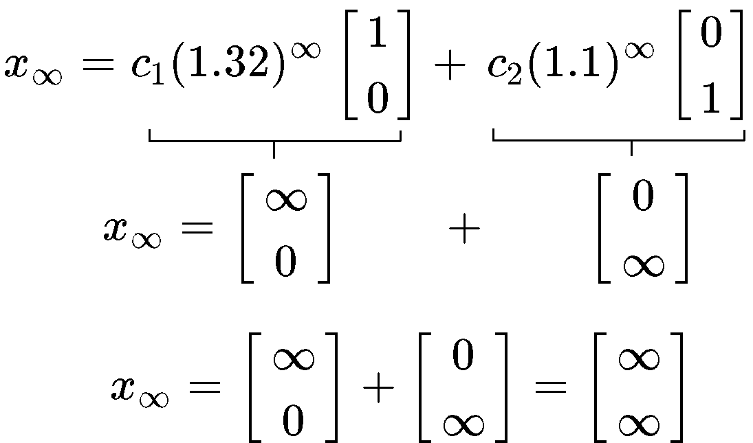
This means that as the transformations progress through time on this system, and they continue to infinity, then the final value of the system will go to infinity too since it just continues to increase every time there is a new transformation.

***
We recommend you to watch all of the videos from this lesson, since the last set of videos talks about a special case called the predator and prey model. Make sure you understand this and remember, you can always asks us if in doubt!.

To finalize this lesson we would like to recommend you to visit the next lesson on an introduction to discrete dynamical systems, which could complement what you have learned today on discrete dynamics with example models.

So, this is it for our lesson on discrete dynamical systems linear algebra, we hope you enjoyed it. See you in the next one!