Image and range of linear transformations
What is a linear transformation
A transformation is a technique in which a vector gets "converted" into another by keeping a unique element from each of the original vector and assigning it into the resulting vector. This process basically maps one vector space into another. There may be different kinds of transformations in mathematics but the case of a linear transformation in linear algebra is that which preserves linear combinations from the original expression to the resulting one, in simple words, it preserves the way addition and scalar multiplication operate from the original vector to the transformed vector. A linear transformation example can also be called linear mapping since we are keeping the original elements from the original vector and just creating an image of it.
Recall the matrix equation Ax=b, normally, we say that the product of A and x gives b. Now we are going to say that A is a linear transformation matrix that transforms a vector x into a vector b (we now call b an image of a linear transformation of x).
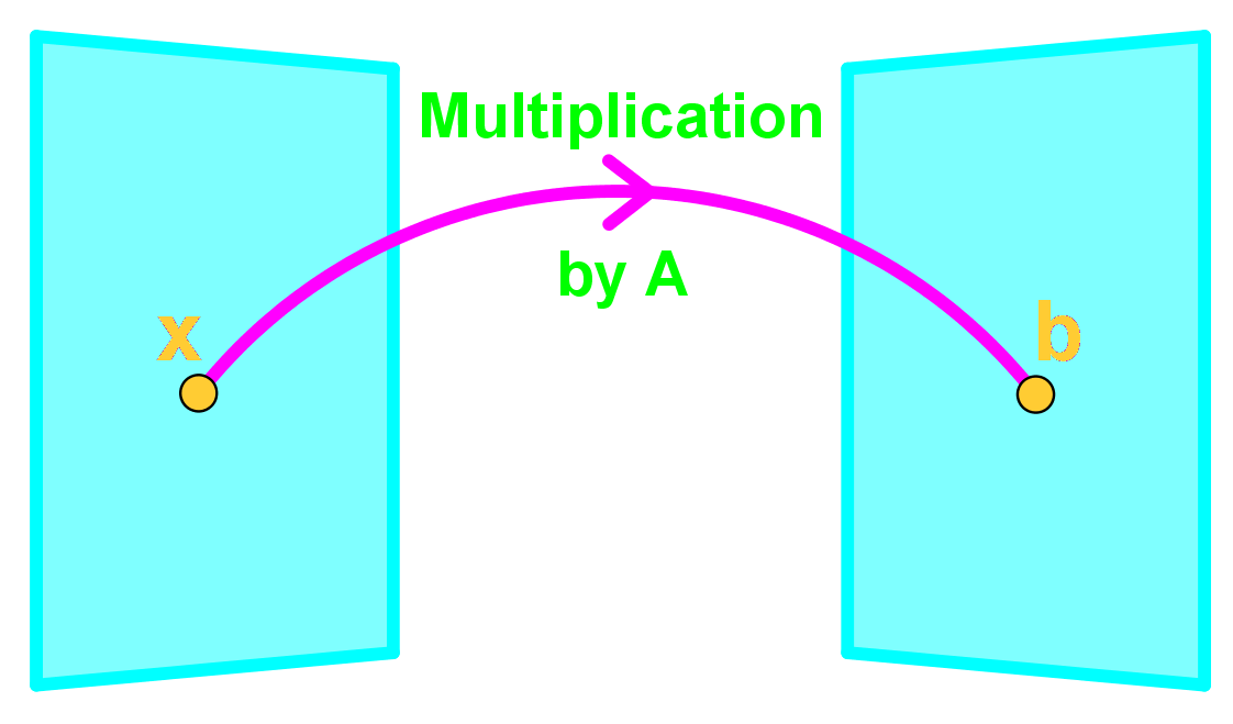
In a sense Ax is a function where if we plug in a vector, then it spits out another vector. If we call this function T(x), then T(x)=Ax
where T is the transformation. Note that T(x) is an image of x since T(x)=b;
How to do a linear transformation
From the linear transformation definition we have seen above, we can plainly say that to perform a linear transformation or to find the image of a vector x, is just a fancy way to say "compute T(x)".
So to compute a linear transformation is to find the image of a vector, and it can be any vector, therefore:
T(x)=Image of x under the transformation T
T(v)= Image of v under the transformation T
And so, if we define T: by T(x)=Ax.Find the image of v under T if:

So our goal is to find T(v)=Av
For that, remember our matrix multiplication guide:

And so, we perform the transformation:

Therefore the image of v is:

But what if the question gives the image and asks you to find the original vector? Let us use the same vectors as above and think how can we do the reverse engineering to obtain v, we start by working out the matrix equation below:

We use what we learned on the lesson about representing a linear system as a matrix, and write down an augmented matrix from our matrix equation above. Then in order to solve for vector v we just have to use row reduction and echelon forms!

And as you can see, we just got the linear transformation proof by reversing the process and obtaining the same vector v we started with:

How to find the range of a linear transformation
We say that a vector c is in the range of the transformation T if there exists an x where: T(x)=c. In other words, if you linearly transform a vector x and c is the result, then it means c is in the range of the linear transformation of x. If c is not a result of the transformation of x, then c is not in the range of the transformation.
For example, if we were to have the vector c shown below.

Is c in the range of the transformation T if the matrix A is the one from equation 1? In order to find out if c is in the linear transformation range we need to compute T(x)=c Ax=c

Notice how we obtained an augmented matrix of a linear transformation so we can solve for the vector x.

And so, a vector x exists! Therefore c is in the range of a linear transformation of x.

Linear transformation examples
Example 1
Consider the matrix below:
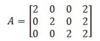
Define the transformation T: by T(x)=Ax. Find the images under T of the two column vectors below:
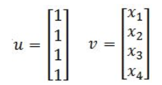
- So we find the images of u and v:

Equation 14: Finding the images of u and v
Example 2
Let's define the transformation T: by T(x)=Ax.
Having:

Find the vector x whose image under T is b,and find out whether x is unique.
The first part of this problem is to find the vector x from the transformation which produces the image b, so in this case we have T(x)=Ax=b. Then we have to prove if x is unique.
- Let us start by solving for x by obtaining the matrix equation Ax=b:

Equation 16: Matrix equation and its corresponding augmented matrix - Then we solve the augmented matrix in order to find x:

Equation 17: Finding vector x
Now, how do we know if x is unique? As you can see from the equation above, is a free variable and therefore, you have infinitely many possibilities as to what the vector x can be. By setting to different values, the transformation T(x)=Ax=b still applies to every single case and so x is not unique!
Example 3
Let's define the transformation T: by T(x)=Ax.
Having
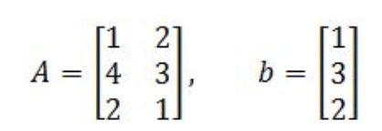
Determine if b is in the range of the transformation T.
- Remember that for b to be an image of the transformation T, then a vector x must exist. And so, we proceed to compute the transformation by writing down its matrix equation and then its corresponding augmented matrix:

Equation 19: Matrix equation and corresponding augmented matrix - Then we solve the augmented matrix in order to find the vector x:

Equation 20: Solving the augmented matrix
And uh oh! We have gotten into an issue, the third row in the augmented matrix gives as a result an inconsistent equation of , the same as saying 0=3 which is of course impossible, and so, this means that a vector x corresponding to this transformation DOES NOT EXIST, and therefore, b cannot be in the range of this linear transformation.
Example 4
Use a graph to plot the vector u and its image under the transformation T. You are given:

- Plotting vector u:
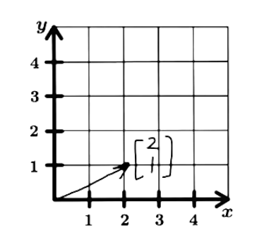
Figure 1: Graphic representation of vector u - If we are given the linear transformation of x as follows:

Equation 22: Linear transformation of x - Let us calculate the linear transformation of u: T(u)=Au

Equation 23: Linear transformation of u - From that we obtained a new vector that we can plot in the graph below:
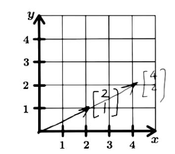
Figure 2: Graphic representation of vector u and its linear transformation
So, what did the transformation do to the vector u?
From the graph you can see that the original vector u doubled in its length, which is the same as having multiplied it by 2. So, linear transformations can change the length of vectors, how much depends on the matrix you are using for the transformation.
Normally, we say that the product of and gives . Now we are going to say that is a transformation matrix that transforms a vector into a vector (we call an image of ).

In a sense is a function where if we plug in a vector, then it spits out another vector. If we call this function , then
where is the transformation. Note that is an image since .
We say that a vector is in a range of the transformation if there exists a where:

 , and let's define
  and
and 


 and its image under the transformation T. You are given that:


