Matrix equation Ax = b
What is a matrix equation
From courses in algebra we known that the definition of an equation is just an "equality". Thus, an equation is a mathematical expression which contains an equal sign inside of it, defining at least two expressions as equal using one or more variables along with numerical values (depending on the need). The variables included in such expressions can also be called unknowns and we solve them by finding the numerical values that make whole equation relationship true.
So, what would be the difference between a regular equation and a matrix equation? This really just comes from the type of notation you are using when writing the equation. A typical equation is written as an algebraic expression, namely: just coefficients and variables defining a mathematical relationship. But we have seen already another type of equation in past lessons: a vector equation, and if you remember from our very last lesson for this course, a vector equation is that where you can distinguish all the coefficients in a system of equations which are related to each variable (there will be an example of this below, or you can just go back to the lesson on linear combinations and vector equations in Rn if you need a review).
And so, a matrix equation is that which uses notation of matrices to express the relationship between its coefficients and its variables. As you will see throughout this lesson, a matrix equation has the capacity to represent more than one simple algebraic equation at the time, and for that, we usually employ them to represent systems of equations.
How to do matrix equations
Since a matrix equation usually represents a multiplication of matrices (as you will see below, some of them are vectors some of them are coefficient matrices) the first thing we need to learn is how to work through and what are the properties of matrix multiplication.
Although we will cover matrix multiplication and its properties extensively in later lessons, the gist of the operation is seen in the next diagram:

Notice how in matrix multiplication the first factor (matrix on the left) must contain the same amount of columns as the amount of rows found in the second factor (the matrix on the right in the multiplication) in order to be doable. Depending on the problem case you are trying to work up, matrix multiplication makes it simple to work with systems of equations and vectors since you have an orderly manner to operate coefficient by coefficient and variable by variable on this way. Let us work in the next three simple examples of matrix multiplication before we continue with our lesson:
Example 1
Compute the following matrix multiplication:

Example 2
Compute the following matrix multiplication:

Example 3
Compute the following matrix multiplication:
This particular multiplication cannot be done, since there are not the same number of columns in the first matrix, as rows in the second one. It is imperative to note that this property of matrix multiplication makes it non-commutative. In other words, you cannot exchange the order in which you multiply matrices and expect to obtain the same result, in some cases you won't even be able to obtain a result if you exchange their order. Take the cases in examples 1 and 2, if you exchange the order in which the matrices are multiplied you would end with multiplications in which the first matrix contains only one column, and the second matrices would have multiple rows, so you would not be able to perform those multiplications, while you had no issue in performing the multiplications as they are right now.
For a matrix equation then, we will usually find the case of a coefficient matrix (a matrix with numerical values only, called coefficients because they may be representing the coefficients from a system of linear equations) being multiplied by a column vector (usually only containing defined variables, but it can contain coefficients as well). Let us take as an example a problem we saw in our last lesson, we start with the system of linear equations below:


For which we can obtain its vector equation and augmented matrix:

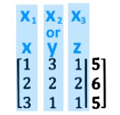
Where the augmented matrix is the representation of such vector equation where the vertical line represents an equal sign. The values in each column of the augmented matrix to the left of the vertical line represent the coefficients for each variable in the system of linear equations, such that (remember the name you give to the variables does not matter):

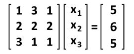
And so, the matrix equation which is equivalent to such augmented matrix is as follows:

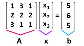
Such matrix equation is one in the form Ax=b! Let us go into the next section to explain it in more detail.
The matrix equation Ax b
If A is an m×n matrix with columns , and if x is in , then the product of A and x is the linear combination of the columns in A using the corresponding entries in x as weights. In other words:

Where b = . Notice that x corresponds to a column vector and A to a coefficient matrix. Using equation 10 as an example to identify the parts of the equation matrix:

And as you might have guessed already, the importance of the matrix equation Ax=b is to provide a way to solve for x (or better said, for the variables in column vector x), which can be easily done by using the three types of matrix row operations and the method of solving a linear system with matrices using Gaussian elimination.
At this point, you may have noticed already that examples 1, 2 and 3 above are pieces of the matrix equation Ax=b, they are actually examples of its left hand side: multiplication Ax only. We know now how to do such simple matrix multiplications and when they cannot be performed, hence, it is time for us to work on exercises where we can see the matrix equation already related to systems of linear equations, such as in equations 7 to 10.
Before we continue to the next section where we will start to practice methodology on how to solve the matrix equation explained above, we need to know a few of its properties. And so, we say that if A is an mn matrix, u and v are vectors in , and c is a scalar, then:
Use such properties while working through matrix equations,reducing and solving augmented matrix in order to find x or any other required processes that will be shown in the methods below.
How to solve a system of equations using a matrix
Let us work through a few different exercises where we'll get the knack of how matrix equations are useful when working with systems of linear equations. The principle in which using a matrix to solve a system of equations is based on, is that every matrix equation Ax=b corresponds to a vector equation which happens to coincide on its solutions, thus we can related them as a system of different algebraic expressions with different variables.
Example 4
We start by converting the system of equations below into a vector equation and then to a matrix equation.


The vector equation can be easily written down by separating all of the different variables (along with their coefficients) in the equations and making them into a distribution of column vectors. This vector equation can then be transformed into an augmented matrix which finally take us into writing a matrix equation in itself. Hint: follow the steps that were described through equations 7 to 10, since is the exact same process that has been taken here. As you can see, we have skipped steps here, but you can see them either following the equations proposed or watching the videos which form part of our lesson. The results are:

Example 5
In the past example we talked about how we can also write the augmented matrix either from a system of algebraic linear equations, or even having the components from the matrix equation Ax=b. For this example we will have such two components (matrix A and b), as follows:

Write the augmented matrix for the linear system, then solve the system and write the solution as a vector. We start by writing the matrix equation Ax=b to form the augmented matrix:

Notice that in order to know how many entries would x have, we have used the rule described in equation 1 for the multiplication of matrices. In other words, if A has two columns, we know x MUST have two rows. Also, if the dimensions mxn of A are 2x2, and the dimensions of b are 2x1, which is a combination of the dimensions of A and x, then x MUST have dimensions 2x1. And so, the augmented matrix results as follows:

Now, to solve matrix equation Ax=b through this augmented matrix, we need to work it out through row reduction and echelon forms. And so, the process goes as:


And out final answer in vector form is:

Solve the matrix equation ax b for x
The process we have seen so far in example 5 starting with A and b, is the general process we follow to solve the matrix equation for x. Let us work through another example of it:
Example 6
Write the augmented matrix for the linear system provided A and b, then solve the system and write the solution as a vector.
Having:

We write the matrix equation and then its augmented matrix form:

We solve augmented matrix from above through row reduction:


And the final vector x is:

Example 7
For this example we will solve matrix equation given the values of A and b below:

Notice how in here we are in the need to solve the equation without knowing the value entries on b, and so, how do we work on this? Let us first start by writing the matrix equation:

In order to obtain the values of b at which this equation has a solution, we need to put the equation in augmented matrix form and then obtain its reduced echelon form:

We stop right there, because we have found a condition for the solution of this equation: only when =0 the matrix equation has a solution, if were to be different than zero, then this would make an equation of 0= any non-zero constant, which is inconsistent! And so, at this point we are left with only one equation (which is the first row of the augmented matrix) in order to solve multiple unknowns! So we so far cannot compute a particular final solution of this equation BUT the solutions exist! There are actually infinitely amount of solutions for this equation as long as the condition is satisfied.
And so, that is how we finalize our lesson for today. We suggest you to take a look at all of the videos included for the lesson since the last part includes a proof of the properties of the matrix equation Ax=b.
For now, we recommend you to visit the next lesson summary containing a section on the matrix equation Ax=b also, this particular lesson on the inverse of a square matrix has an interesting section at the bottom where you can see how Ax=b can be used to solve systems of linear equations and to calculate x through inverting A.

If we were to say that , then basically:
which we see b is a linear combination of . You will see questions where we have to solve for the entries of again, like last section.
We say that an equation in the form of is a matrix equation.
Properties of
If is an matrix, and are vectors in , is a scalar, then:
1.
2.


 and
and  . Show that the matrix equation


