In this section we will learn about matrix row operations. There are three types of matrix row operations: interchanging 2 rows, multiplying a row, and adding/subtracting a row with another. Each notation for this is different, and is displayed in the note section. First, we will look at questions which involve all three types of matrix row operations. Then we will look at more slightly advanced questions that involve using 2 matrix row operations.
The three types of matrix row operations
Matrix row operations refer to arithmetic operations, or combinations of such operations that can be applied to the rows of a matrix (it doesnt matter the type of matrix in question) in order to solve a system of linear equations.
Simply said, matrix row operations are the ones used after you have converted a system of linear equations into a matrix equation, to then simplify it as much as possible in order to find the solutions to the variables in the system. The complete algorithm (steps to be followed) for solving systems of equations through row operations is called the Gaussian elimination.
The last lesson focused on representing a linear system as a matrix, but after having the augmented matrix containing such system, how do we solve it? In our next lesson we will focus on exactly that: solving a linear system with matrices using Gaussian elimination. But before we are ready, we need to learn about the basic row operations and the combinations that can be applied to the matrix being worked on. Then, row operations matrix are our topic for today! Something important to know is that although we will be working on augmented matrices in order to solve systems of linear equations, you can compute such row operations on any type of matrix.
Matrix elementary row operations
There exist three types of elementary matrix row operations:- Interchanging two rows
- Multiplying a row by a constant (any constant which is not zero)
- Adding a row to another row
From those three, we can have combinations, such as multiplying a row by a nonzero constant to then add it or subtract it to another row, or maybe exchange them. Elementary row operations on an augmented matrix never change the solution set of the equations, in other words, even though you are operating on the matrix, the matrix obtained after every computation is equivalent to the one you had before.
In order to have a clearer picture of how these matrix elementary row operations work, let us expand our explanation of each of the three basic ones:
1. Interchange of rows
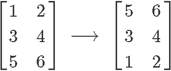
We interchanged the row 1 and row 3. Another way of saying this is: , where represents the row one (the first row from top to bottom) and is row three (the third row from top to bottom). Exchanging the rows of a matrix produces an equivalent matrix, which means that the algebraic relationship (or proportionality) remains the same.
If you think about it, interchanging two rows in a matrix which represents a system of linear equations means that you are just exchanging the order in which the equations are listed in a system, which of course, has NO effect on the solutions of the variables in the equations.
Remember from our past lesson, that the rows in an augmented matrix coming from a linear system of equations each represents an equation from the system, therefore, the order in which you list a system of equation makes nothing on the proportional relationship expressed through them about their variables.
To make this a little bit clearer, let us look into the system shown in the second example exercise of our past lesson:

On this system, you have two equations, each transcribed as a row in the matrix notation. Would it make any difference in the solutions for x and y if we were to put the second equation on top instead? This would produce a matrix in which you would have the second row of equation 2 as the first row in the matrix. The answer is: NO. It really does not matter in which order you list the equations in a system, and thus, it does not matter how you transcribe them in a matrix equation as long as you keep them in rows, so, you can only exchange a complete row with another complete row (in other words, you cannot exchange the order of the columns because this would change the coefficient associated to a variable in an equation, thus changing the equations).
2. Multiplying a row by a non-zero constant

On this elementary row operations matrix process we have multiplied the non-zero constant 3 to the first row of the original matrix. Such operation is represented by .
As you can see, this multiplication will affect each coefficient in row one in the same way one would apply such factor to all of the terms in an equation which has been multiplied by a constant.
Let us see this effect going on for an augmented matrix, we take the system represented in the exercise example number 8 from last lesson:

If we were to multiply the non-zero constant 2 to the first row of the matrix, this would mean the resulting equation for this row would be: . Notice how such multiplication for a non-zero constant (any non-zero constant) would not make a change in the value of the variables when solving for them because the proportionality relationship remains. This is an important thing to notice, since it brings to our attention how this row operation makes an emphasis on the constant multiplied being different than zero. If instead of a non-zero constant we were to multiply the first row by zero, this would mean we would end up with an equation for that row equal to , which would actually leave us with only two equations to solve a system with three unknown variables, thus making it not possible to solve anymore.
3. Adding a row to another row

Where we have replaced row 2 for the result of the addition of rows 2 and 1. Such operation is represented as: →. You can do this with any two rows (adding them of subtracting them from one another and replace one of them with the result).
Having seen the three basic row operations it is worth noting that you can combinations of these three types of matrix row operations in order to manipulate the coefficients on a matrix to your convenience.
Probably the more complicated scenarios will come when you have to work through a combination of augmented matrix row operations, meaning, whenever you will have to apply a combination of the elementary operations seen above into an augmented matrix. But worry not, in the next section we will focus on showing examples of such processes so you can practice.
Remember that the purpose of row operations on augmented matrices is to simplify the matrices as much as possible in order to solve for the values of the variables in the system of equations they represent. Such simplified matrix forms are what we call the echelon form and the reduced echelon form, and they are the key for finding the final solutions to the equations in the system. Different sequences of row operations can lead to different echelon forms for the same matrix, we will work through them and cover such topics as the elementary matrix, row reduction and echelon forms in the next lessons of our Linear Algebra course, for now we will focus on just learning the elementary row operations.
Before we continue with the exercise examples of this lesson, we recommend you to take a look into these notes on elementary row operations for matrices which could serve to complement todays lesson, plus it gives a little introduction on matrices and systems of equations.
Matrix row operations examples
On this section we will see two examples of matrices on which we will compute a few times to apply the three elementary matrix row operations (for the first example) and then a combination of the elementary row functions on the second example.Notice that for each operation in each example we will start from the original matrix and then apply the operation concerning to that case (in other words, the operations will not be cumulative for a single matrix, but will start from the original each time). Although you will work with cumulative row operations in later lessons, for now the important thing is for you to learn how to apply the basic operations and their possible combinations from the beginning. In later lessons you will continue to practice such operations and making them a cumulative process, but there will be plenty of time and examples to practice on when that time comes.
Observe how the two examples below do not contain augmented matrices, this has been selected on purpose so you know the row operations can be applied to any type of matrix. When solving systems of linear equations in later lessons we will mostly be using augmented matrices.
Example 1:
You are given the following matrix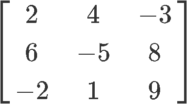
Perform the following matrix operations:
a)

b)

c)

d)

e)

f)

Again, notice that during this example and its multiple cases, we have only used the most elementary three row operations possible, but in most cases is much more practical to combine them in order to reduce the matrix into a simplified one much faster. In the next example, we will be looking into an example for which we will be applying combinations of row operations.
Example 2
You are given the following matrix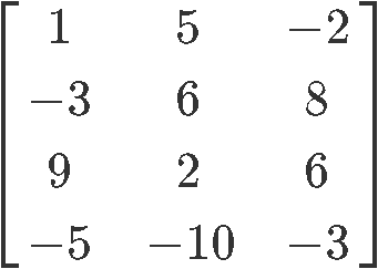
Perform the following matrix operations:
a)

b)

c)

d)

If you are ever in doubt that such matrix row operations generate a matrix which is not equivalent, you can always prove it on your own, take the matrices we have used in these examples and convert them into the algebraic notation to obtain the systems of linear equations corresponding to each of them. Having such systems, solve for the values of their variables using other method we have learned in algebra before, such as solving systems of linear equations by substitution, elimination or even graphing. The proof process will serve for a lot of practice, thus we highly recommend it.
Matrix row operations are the basis for row reduction, the method we have mentioned before (also named Gaussian elimination), thus after this lesson you are ready to start working on cumulative row operations on matrices in order to reduce them to echelon forms and obtain the values of the variables in the system. Although lessons like this one can seem tedious and repetitive, it is imperative you have well settled basis for what is coming next.
Now get ready, we are finally going to solve the systems of linear equations we have been talking about. See you in the next lesson!
The first type of matrix row operation is that we are allowed to switch any rows you want. For example,

We interchanged the row 1 and row 3. Another way of saying this is .
The second type of matrix row operation is that we can multiply a row by a non-zero constant. For example,

We multiplied each entry in row 1 by 3. Another way of saying this is .
The third type of matrix row operation is that we are allowed to add and subtract a row with another. For example,

Row 2 is the sum of row 2 and 1. Another way of saying this is →.

We interchanged the row 1 and row 3. Another way of saying this is .
The second type of matrix row operation is that we can multiply a row by a non-zero constant. For example,

We multiplied each entry in row 1 by 3. Another way of saying this is .
The third type of matrix row operation is that we are allowed to add and subtract a row with another. For example,

Row 2 is the sum of row 2 and 1. Another way of saying this is →.


