Step Functions
What is a step function?
The main characteristic of a step function, and the reason why it truly looks like a staircase doodle, is that this function happens to be constant in intervals. These intervals do not have the same value and we end up with a function which "jumps" from one value to the next (following its own conditions) in a certain pattern. Every time the function jumps to a new interval it has a new constant value and we can observe the "steps" on its graphic representation as horizontal lines. Take a look at the graphic representation below for a typical step function where is plain to see how the name of the function came about.
Notice from the figure above that we can also define a step function as a piecewise function of constant steps, meaning that the function is broken down in a finite number of pieces, each piece having a constant value, in other words, each piece is a constant function.
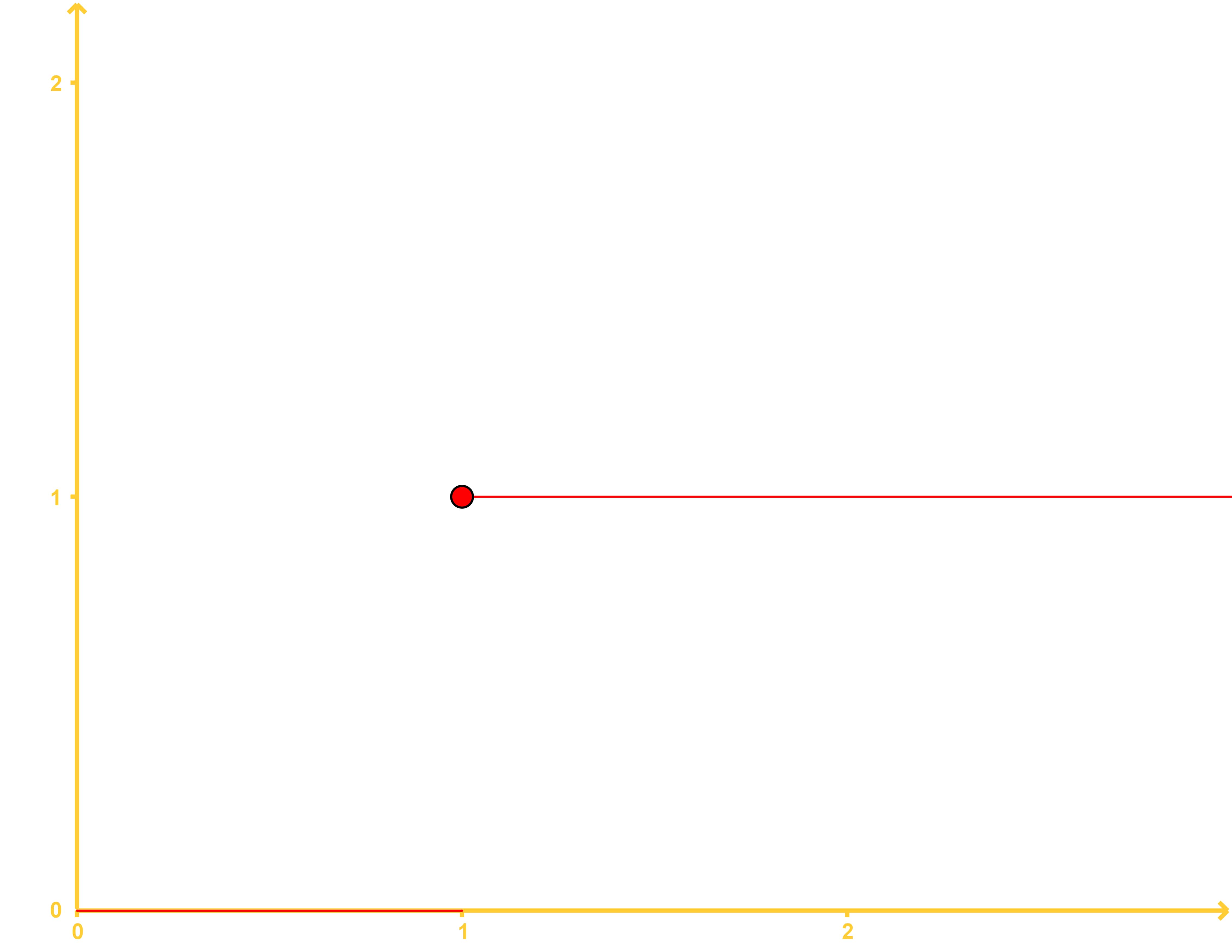
When talking about step functions we cannot forget to talk about the Heaviside function also known as the unit step function. This is a function that is defined to have a constant value of zero up to a certain point on t (the horizontal axis) at which it jumps to a value of 1. This particular value at which the function jumps (or switches from zero to one) is usually taken as the origin in the typical coordinate system representation, but it can be any value c in the horizontal axis.
Consequently, the Heaviside step function is defined as:

Where c represents the point at t in which the function goes from a 0 value to a value of 1. So, if we want to write down the mathematical expression of the heaviside function depicted in figure 3, we would write it as: u3(t). Notice how we only wrote the math expression using the first type of notation found in equation 1, this is because that notation happens to be the most commonly used and is also the one we will continue to use throughout our lesson. Is still important though, that you know about the other notations and keep them in mind just in case you find them throughout your studies.
From its definition, we can understand why the Heaviside function is also called the "unit step" function. As it can be observed, a Heaviside function can only have values of 0 and 1, in other words, the function is always equal to zero before arriving to a certain value t=c at which it "turns on" and jumps directly into having a value of 1, and so, it jumps in a step size of one unit.
Notice how we have used the phrase "turning on" to describe the process of the unit step function to jump from a zero value to a unit value, this is a very common way to refer to Heaviside step functions' behavior and interestingly enough, it is all due to their real life usage and comes from the reason why they were invented. Historically, physicist, self-taught engineer and mathematician Oliver Heaviside, invented Heaviside step functions in order to describe the behaviour of a current signal when you click the switch on of an electric circuit, thus, allowing you to calculate the magnitude of the current from zero when the circuit is off, to a certain value when is tuned on.
There is an important note to clarify here. Electric current does not magically jump from a zero value to a high value. When having a constant current through a circuit, we know that this constant value obviously started off from zero from when the circuit was off and then it arrived until a certain value after gradually increasing in time, the thing is that electric current travels at a very high speed, and so it is impossible for us (in a simple everyday life setting) to see this gradual increase of the current from zero to its final value since it happens in a very short instant of time, and so, we take it as a "jump" from one value to the next and describe it accordingly in graphic representations.
Heaviside function properties
Although the Heaviside function itself can only have the values of 0 or 1 as mentioned before, this does not mean we cannot obtain a graphic representation of a higher jump using Heaviside step functions. It is actually a very simple task to obtain a higher value since you just need to multiply it for any constant value that you want to have as the size jump, in other words, if you have a step function written as 3u5(t) in here you have a step function which has a value of zero until it gets to a value of t=5, and which point, the function has a final value of 3. This can be seen in the figure below:
One of the greatest properties of Heaviside step functions is that they allow us to model certain scenarios (like the one described for current in an on/off circuit) and mathematically be able to solve for important information on these scenarios. Such cases tend to require the use of differential equations and so here we have yet another tool to solve them.
Being this a course on differential equations, the most important point of this lesson is to give an introduction to a function which will aid in the solution of certain differential equations, such tool will be used along others seen before, such as the Laplace transform. This will serve to come up with important formulas to be used and to be prepared for the next lesson in which you will be solving differential equations with step functions.
We will talk a bit more about this on the last section of this lesson, meanwhile for a review on the definition of the unit step function and a list of a few of its identities, we recommend the next Heaviside step function article.
Heaviside step function examples
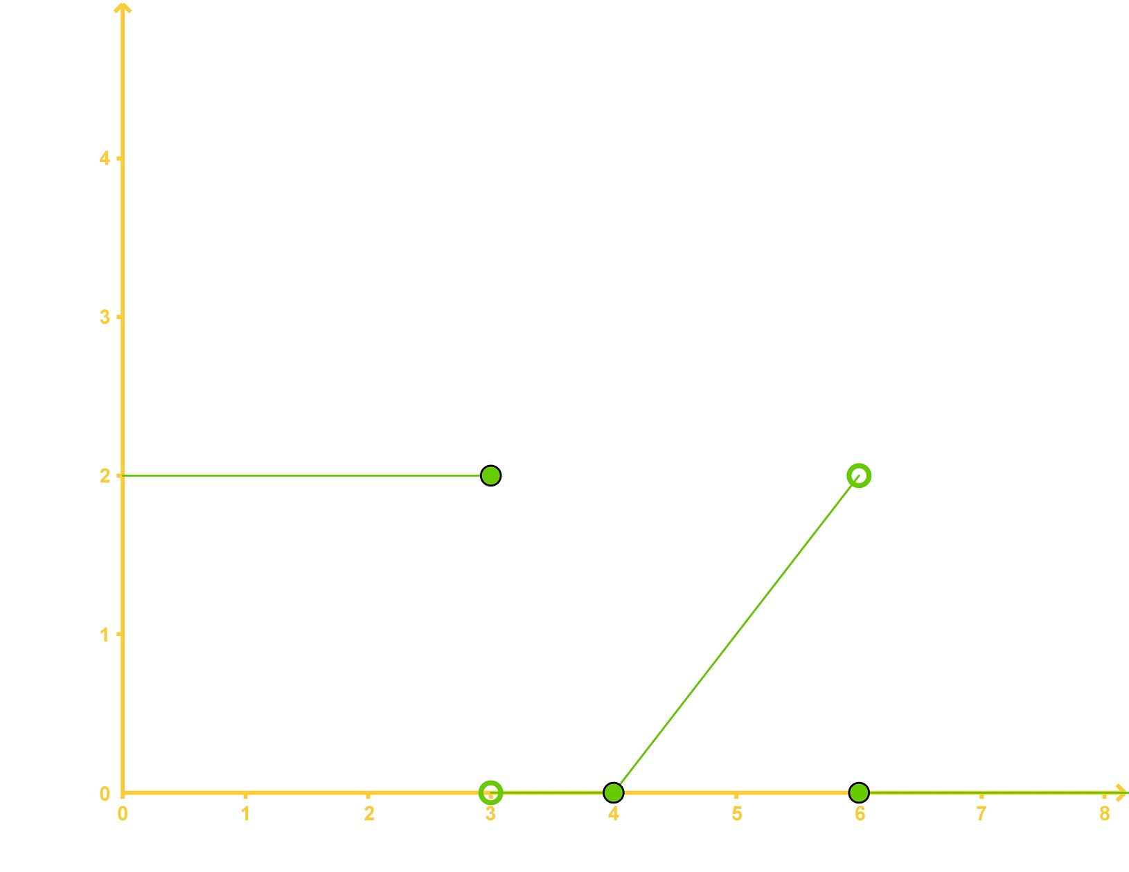
Let us take a look into an example in which you will have to write all of the necessary unit step functions in order to completely describe the graphic representation found in figure 5.
Example 1
Write the mathematical expression for the following graph in terms of the Heaviside step function:
Let's divide this in parts so we can see how the functions of the graph behave at each different value given. And so, we will write a separate expression for each of the next pieces: for t < 3, for t=3 to t=4, for t=4 to t=6 and for t>6.
-
For t < 3: Notice that this is a regular Heaviside function in which c=0, multiplied by a 2 in order to obtain the jump of 2 units in size. This would fit the requirement of the function being zero for all negative values of t, and then to have a value of 2 for values of t from 0 to 3. And so, the expression is: 2uo(t)=2. -
For t=3 to t=4: In this range we have to cancel the unit step function that we had before, that means we need a negative unit step function in here but this one will start to be applied at t=3 and will have to be multiplied by 2 again in order to cancel the value of the previous expression. Thus, our expression for this part of the function is: -2u3(t).
-
For t=4 to t=6: If we weren't to add any function at t=4, the value of the function would remain as zero to infinity since the second function cancelled the first one, but instead, we see in the graph that we have a diagonal line increasing one unit step size for each one unit of distance traveled on t.
Thus, since the function is increasing at the same rate as t, we could easily multiply a new unit step function which starts at 4 by t and be over with, this would produce a diagonal line following the same behavior. The problem is that just multiplying u4(t) by t would produce a line that would come out of the origin instead of t=4, and for that, we need to multiply the unit step function by (t-4) so the function starts at the same time as the unit step function will be applied (which is at t=4). And so the expression is: (t-4)u4(t).
Notice (t-4)u4(t) produces the values for y of: 0 (when t=4), 1 (when t=5) and 2 (when t=6), which is what the graph requires.
-
For t > 6: For this last piece of the graph should be already easy that we just need to cancel our last function in order to have a value of zero back to the graph. For that we use a negative unit step function which starts at t=6, and which should be multiplied again by (t-4). And so, the expression to cancel our last one and completes the graph is: -(t-4)6(t).
We add all of the four pieces of function we found to produce the expression that represents the whole graph shown in figure 5:

Equation for example 1: Mathematical expression for the graph in figure 5
Due to this particular example having multiple step function samples, we continue onto the next section to work on more complicated problems.
If you would like to continue practicing how to write down Heaviside step functions, we recommend you to visit these notes of step functions for more Heaviside function examples along with a little introduction. Notice these notes also introduce the topic for our next section: unit step function Laplace transforms and the overall use of the Laplace transform when associated to Heaviside functions.
Laplace transform of Heaviside function
You have already had an introduction to the Laplace transform in recent past lessons, still, at this time we do recommend you to give the topic a review if you think it appropriate or necessary. The lesson on calculating Laplace transforms is of special use for you to be prepared for this section.
Let us continue with the Heaviside step function and how we will use it along the Laplace transform. The Laplace transform will help us find the value of y(t) for a function that will be represented using the unit step function, so far we have talked about step functions in which the value is a constant (just a jump from zero to a constant value, producing a straight horizontal line in a graph) but we can have any type of function to start at any given point in time (which is what we represent with t mostly).
What are we saying? Well, think on the graphic representation of a function, you can have any function, with any shape, but this special case comes from the fact that the function will be zero through time, until a certain point in which the signal will turn on, and then it will "jump" into this "any shape" function behavior. This is what we call a "shifted function" and this is because we can think of any regular function graphed, and then saying "oh but we want this function to start happening later" and we "switch" it to start at a later point in time (at t=c).
Since these shifted functions will be equal to zero until at certain point c in which they will "turn on", they can be represented as:
The shifted function then is defined as:

Now let's see what happens when we take the Laplace transform of a shifted function!
First, remember that the mathematical definition of the Laplace transform is:

Therefore the Laplace transform for the shifted function is:

Notice how the Laplace transform gets simplified from an improper integral to a regular integral where you have dropped the unit step function. The reason for this is that although the range of the whole Laplace transform integral is from 0 to infinity, before c (whatever value c has) the unit step function is equal to zero, and therefore the whole integral goes to zero. After c, the unit step function has a value of 1, and thus, we can just take it as a constant value of 1 multiplying the rest of the integral, which range is not from c to infinity.
Continuing with the simplification of the Laplace transform of the shifted function, we set x = t - c, which means that t = x+c and so the transformation looks as follows

By making the integral to be in relation to one single variable rather that a t-c term, we have simplified this transformation so we could obtain a quickly manageable formula we can readily use with future problems and our already known table of Laplace transforms from past lessons.
Having solved equation 5 makes it easier to obtain another important formula: the unit step function Laplace transform. Notice, not the transform for a shifted function, but the Laplace transform of the unit step function (Heaviside function) itself and alone.

If you notice, equation 5 was useful while obtaining equation 6 because taking the Laplace transformation of the Heaviside function by itself can be taken as having a shifted function in which the f(t-c) part equals to 1, and so you end up with the Laplace transform of a unit step function times 1, which results in the simple and very useful formula found in equation 6.
Now let us finish this lesson by working on some transformation of a unit step function examples.
Example 2
Find the Laplace transform of each of the following step functions:

-
Applying the Laplace transform to the function and using equations 5 and 6 we obtain:

Equation for example 2(a): Computing the Laplace transform on the unit step function (part 1) -
Using equation 5, we set x=t-c (for this case x=t-5) and work through the transformation on the second term of the last equation:

Equation for example 2(b): Computing the Laplace transform on the unit step function (part 2) Notice that in order to solve the last term, we used the method of comparison with the table of Laplace transforms. You can find such table on the past lessons related to the Laplace transform.
-
Now let us solve the third transformation (remember we set x = t-c, which in this case is x=t-7):

Equation for example 2(c): Computing the Laplace transform on the unit step function (part 3) -
Now we put everything together to form the final answer to the problem:

Equation for example 2(d): Computing the Laplace transform on the unit step function (part 4)
Example 3
Find the Laplace transform for each of the following functions in g(t):

-
Now we use equation 5 and set up x=t-c to solve the Laplace transform:

Equation for example 3(a): Computing the Laplace transform of the unit step functions (part 1) -
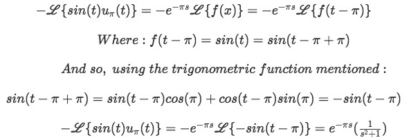
We separate the two terms found on the right hand side of the equation, and solve for the first one (for this case x=t-) using the trigonometric function: sin(a+b)=sin(a)cos(b)+cos(a)sin(b).
Therefore:

Equation for example 3(b): Computing the Laplace transform of the unit step functions (part 2) -
Now let us solve the second term, where x = t-4, therefore, t=x+4:

Equation for example 3(c): Computing the Laplace transform of the unit step functions (part 3) -
Putting the whole result together:

Equation for example 3(d): Laplace transform of g(t)
And now we are ready for our next section where we will be solving differential equations with what we learned today. If you would like to see some extra notes on the Heaviside function and its relation with another function which we will study in later lessons, the Dirac delta function, visit the link provided.
A Heaviside Step Function (also just called a "Step Function") is a function that has a value of 0 from 0 to some constant, and then at that constant switches to 1.
The Heaviside Step Function is defined as,


The Laplace Transform of the Step Function:
These Formulae might be necessary for shifting functions:


