Margin of error
In order to understand what a margin of error for a statistic of a sample population is we need to have a little review and remember the concepts of confidence level, confidence interval and critical values.
As seen in our lesson on confidence levels and critical values, the confidence level of a statistic refers to the amount of trust you have on your own experiment and/or analysis to yield results that match with that of the actual population. In simple words, the confidence level is the percentage of times in which an experiment can be repeated and in which it will yield a result truthful to the actual characteristics of the population that is being studied. The beauty of such confidence is that it comes from sample analysis alone.
A higher level of confidence means that the characteristics being depicted in a statistical study are reliable and represent the actual population in question; while a very low confidence level means that the results cannot be trusted. But remember, a statistic with a 100% confidence level does not exist because a 100% level of confidence would mean that every time the sample analysis of a population is repeated the result is exactly the same (thus is the true value) and this can only be obtained for certain when the complete population is used in the analysis and not simply a random sample.
Just as important, we have that the confidence interval comprises the range of values of a confidence level. In other words, the confidence interval is just like its name portrays: an interval, that contains within itself, the confidence level of a sample analysis.
To have a better idea of what the confidence level and confidence interval are, let us use the empirical rule of statistics, which gives us the approximation of data percentage found in different regions of a normal distribution, to observe them clearly:

The left hand side of figure 1 shows the empirical rule, also called the 68-95-99.7 rule because it provides the confidence levels containing approximately 68%, 95% and 99.7% of the data points from a standard distribution calculated from a sample analysis. This means that we have here, the confidence levels of 68.26, 95.44 and 99.72, thus, we also have their confidence intervals:
- For the confidence level of 68.26%, its confidence interval goes from a negative standard deviation to a positive standard deviation from the mean.
- For the confidence level of 95.44%, its confidence interval goes from two negative standard deviations to two positive standard deviations from the mean.
- For the confidence level of 99.72%, its confidence interval goes from three negative standard deviations to three positive standard deviations from the mean.
Then, the critical value associated to a confidence interval is simply the point on the horizontal axis of a graph marking the start of the confidence interval itself.
Mathematically speaking, a confidence interval is given by: or equivalently:.
Where:
the critical value
the point estimate, a sample estimate
the population proportion
sample size
Remember the point estimate is defined as follows:
Where:
the point estimate or the sample estimate
sample size
number of successes in the sample (individuals with the desired trait)
Therefore, to summarize what is shown in figure 1 on its right hand side, we have that: The confidence level in cyan color occupies 68.26% of the total area under the curve or simply said, it covers an area of 0.6826 out of the total. Its confidence interval spreads to one standard deviation from the mean on both sides and it starts with the critical value of -1.
And so, what is the margin of error then? Let us go to the next section of this lesson and find out!
What is a margin of error?
The margin of error is how much your result from an statistical analysis could differ from the true value, therefore, it provides us with the amount of error coming from the random sampling analysis. The most important things to remember about margin of error statistics are:
- The bigger the sample being studied from a population, the smaller the margin of error will be.
- The lower the margin of error, the better the result from our analysis; meaning that our result is closer to the true value statistic of the population.
- The margin of error is always a positive value when not all of the population has been sampled.
We can relate our margin of error definition with concepts we are already familiarized with:
For example, since a confidence interval is defined as or we can see how is simply the margin of error for the statistic.
How? happens to be the amount of possible random error that you have for the sample analysis. By using the sample estimate as the middle point, refers to half the width of the confidence interval and provides a range of possibilities nearby that allows for this margin of error. In other words, the margin of error is just the amount you either subtract or add from the point estimate which produces the confidence interval (and thus, ).
Therefore, if you want to find the margin of error of an statistic, the only thing you need to do is to calculate the half size of its confidence interval, or , using equation 1. In other words, equation 1 happens to be the formula for margin of error!
How to calculate the margin of error
Let us take a look at a few examples:
Example 1
A sample of = 750 is polled from a population. The sample has a critical value of = 1.75 with a point estimate of = 0.44. What is the margin of error for estimating the population proportion?
The first thing to calculate the margin of error in this case is to find the confidence interval using equation 1. Thus, having = 1.75, = 0.44 and = 750 we compute as follows:
And so, we can conclude that if the point estimate for the statistic on this example problem is equal to 0.44, then the margin of error for estimating the population proportion is 0.03 which means that the population proportion could be any value within 0.41 to 0.47.
Example 2
A ski mountain (Whistler) sees 25,000 visitors a day. The company running the ski mountain wishes to estimate the number of snowboarders who visit this mountain daily. The company surveys 100 people who are visiting the mountain and finds that 43 of them are snowboarders. If the company desires a confidence level of 0.90 in their calculations, what is their margin of error?
In order to make the margin of error calculation (using equation 1) we have to have the following data:
= the critical value
= the point estimate, a sample estimate.
= the sample size.
= number of successes in the sample (individuals with the desired trait)
From this, the sample size has been provided: = 100 (since there were 100 people surveyed) and the number of individuals which were snowboarders (the desired trait) out of this sample is equal to = 43.
Using this information we can calculate the point estimate using equation 2 as follows:
Now, we are left with the task of obtaining the critical value using the confidence level of 0.90.
From past lessons we know that the steps for finding a critical value when knowing the confidence level are as follows:
- Draw the standard normal curve with the proper confidence level being portrayed and identify the limits of the confidence interval.
- If you are looking at a two-sided confidence level centered at the mean, then you need to calculate the area under the standard normal curve which doesnt belong to the confidence level (this area is called ).
- You will have half of on the left, and half of it on the right.
- Calculate the value of /2 and then use this value to find the corresponding z-value from the z-table. Notice this is done, since this /2 value is equal to the area under the curve on the left tail of the distribution.
- This is your critical value (the value of z at which the confidence interval has its lower limit).

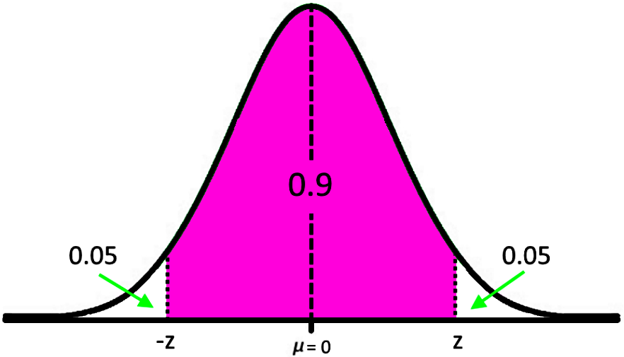
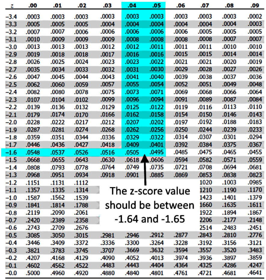
Notice that since the confidence interval encloses an area under the curve which is 90% of the total area under the curve, and since this area is centered on the mean; then, each little piece on each side outside of the confidence interval must account for 5% of the area under the curve. This means that there is a probability of 5% for a data point to be within the area under the curve in the left hand side of the confidence interval, and we can use this bit of information to look for the z-score which produces this probability of 0.05 just as shown below:

And so, we have that the z-score value delimiting the confidence level on the left hand side is approximately -1.645, which means that the critical value will be:
Now that we finally have all of the bits of data needed in order to calculate the margin of error, we just follow equation 1 and compute :
Which means that our margin of error is of 8%, and thus, if our point estimate of snowboarders visiting the park daily was 43, that means that daily, we have an estimation that there could be from 35 to 51 snowboarders.
This means that our final answer is that, we are 90% confident that there are from 35% to 51% snowboarders among the total amount of visitors to the park a day. And out margin our error runs from 0.35 to 0.51.
Example 3
A survey is done linking the number of concussions a season to hockey players. The NHL consists of 700 players and we wish to have a confidence level of 0.95 (corresponding to a critical value of ). Let us assume that the point estimate will be for every sample taken.
a) What is the margin of error, if 20 players are sampled?
In this case, we have the following data:
the critical value
the point estimate, a sample estimate.
the sample size
And so, using the margin of error formula we calculate:
Therefore, our margin of error in this case is about 4.9%
b) What is the margin of error, if 100 players are sampled?
In this case, we have the following data:
the critical value
the point estimate, a sample estimate.
the sample size
And so, using the margin of error equation we calculate:
Therefore, our margin of error in this case is about 2.2%
As you can see from the results in part a and b of this problem, as the sample size increases, The margin of error decreases.
c) What is the margin of error, if all 700 players in the NHL are polled?
In this case, we have the following data:
the critical value
the point estimate, a sample estimate.
for this case the sample size comprises the whole population.
And so, we calculate:
Therefore, our margin of error in this case is about 0.8%, a very small margin of error! Why? Because you are taking into account every single individual of your population, thus, your final result should be equal (or at least VERY similar) to the true value of the number of concussions in a season to hockey players.
So, now that you have learned the relationship between a confidence interval and the margin of error of a statistic (the margin of error of a confidence interval is the error from biased sampling methods), we are left with recommending you some extra resources for your study time!
First, we suggest you to check out this presentation on confidence intervals which provides a clear definition of the margin of error and how this is related to the other concepts we have studied before.
Also, we would like to recommend you this article named Explained: margin of error which gives an interesting insight into how statistical data are reported (or misreported) in political campaigns/media by showing a particular example from the past.
With this we conclude our lesson for today, we hope you enjoyed it, see you on the next one!


