Measures of relative standing
A measure of relative standing is a way to describe the relationship between a specific value in a data set with the rest of the values in the set, or, a way to compare values coming from different data sets with each other. Specifically, a measure of relative standing refers to mathematical tricks that allow you to scale a data set and its distribution in a way that you can meaningfully compare this data in many ways (be it within itself, or with other proportionally scaled data sets); for that, a measure of relative standing focuses on the relative position of a data value within the data set and they are also called measures of location or measures of position.
The three basic measures of relative standing are the z-score (also called the standard score), the percentiles (and their percentile rank) and quartiles.

What is a z score?
The z score let us know of how far away a data point is from the mean of its set, in units of the standard deviation of the set. In other words, once you have calculated the mean of a data set and its distribution, you can calculate how many of these standard deviations separate each particular data point from the mean, that is the z score for each value.
• What does z score mean
The process can get quite complicated, so let us first start with the basic calculation for the z score, and once we have learned more about the normal distribution we can come back to the use of the z score for higher difficulty, unrelated data set, comparisons.
• How to calculate a z score
Where:
= Z score
= to the data value
= mean of the data set
= standard deviation of the data set (which is a population in this case)
Equation 1 is also called the standard score formula and it represents the mathematical z-score definition.
Accordingly, the z score equation for a sample is defined as:
Where:
= Z score
= to the data value
= mean of the data set
= standard deviation of the data set (which is a population in this case)
Let us look at the usage of the z score in the next example:
Example 1
Using Z-score to Compare the Variation in Different Populations, look at the next case:Charlie got a mark of 85 on a math test which had a mean of 75 and a standard deviation of 5. Daisy got a mark of 75 on an English test which had a mean of 69 and a standard deviation of 2. Relative to their respective mean and standard deviation, who got the better grade?
We need to calculate the z-score for the grades of Charlie and Daisy and see who (if any) was among the best on their classes. We have the following information:
= Z score for Charlie
= 85
= 75
= 5
= Z score for Daisy
= 75
= 69
= 2
Therefore, using the z score formula from equation 1, we calculate the z scores for each student and find:
So after we have gotten the corresponding z scores, how do we know which of their grades is better? Well, the results from equation 3 tell us that Charlie got a test mark 2 standard deviations higher than the mean of the class, while Daisy got a mark that is 3 standard deviations higher than the mean in her class. Therefore, proportionally speaking, Daisy did better within her class in comparison to Charlie.
NOTICE: Daisy did better WITHIN her class, in comparison to how Charide did WITHIN his class; thus, the z score calculation let us know how they proportionately did within their classes (meaning that Daisy was probably among the people with the highest marks for that test in her class). This does not mean that Charlies grade is absolutely worse than Daisys. If taken as an absolute value only, Charlie still got a higher mark compared to Daisy; still, proportionally speaking, it appears that people in Charlies class got higher marks too and so he wasnt among the very highest marks in his class.
What is a percentile?
Now let us talk about another measure of relative standing, the percentile. Percentiles indicate the percentage of data outcomes in a set which fall under a certain value.
• How do percentiles work
• How to calculate percentiles
Let us look at an example so you see the process of finding percentiles in action:
Example 2
Sidney is taking a biology course in university. She got a mark of 78% and the list of all marks from her class (including her mark) is given by {56, 83, 74, 67, 47, 54, 82, 78, 86, 90}.- What percentile did she score in?
- Sidneys friend Billy knows he got in the 70% percentile, what was his mark?
First we order the scores from lowest to highest: {47, 54, 56, 67, 74, 78, 82, 83, 86, 90}. Notice we put Sidneys score in bold. Now, solving for the percentile Sidney scored in, we use the percentile formula shown in equation 4:
So we have that Sidney scored in the 50th percentile (or above the 50%).
Now to answer the second question of this problem, let see what is Billys mark if he is in the 70th percentile: Using the percentile equation (equation 4) we solve for the number of data points less than X so we can then go and check back which score meets this condition in the set:
Therefore, there are 7 data values in the set before Billys score, which means Billy got a 83% in his Biology course.
What are quartiles
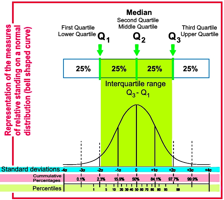
Just as its name indicates, a quartile focuses on dividing the data distribution into four parts, where each quartile is the specific point marking the division between the first quarter and the second, the second quarter and the third or the third quarter and the fourth. In simple words, quartiles are values that divide a data set into quarters after the data set has been ordered; each quartile has a name and they are: and .
Where:
= splits the lowest 25% of the sorted data
= Median=splits the lowest 50% of the sorted data
= splits the lowest 75% of the sorted data
The middle 50% of the data in the data set and its proper distribution comprises the interval named the interquartile range, which is equal to subtracting the first quartile from the third quartile.
Do not confuse a quartile with a quarter, while each quarter refers to the whole fraction of the data representing 25% of it, the quartile is the point that marks the division between one quarter and the other.
• How to calculate quartiles
Let us explain the method to calculate quartiles with the next example:
Example 3
Find the quartiles for each data set: a) {9, 3, 7, 5, 2, 8, 12}
We first find the median, for which you have to order the data values from lowest to highest first and then find the value in the midpoint.
The media represents the second (or middle) quartile, for this case .
Then we just obtain the median for each half of data values on the left and right of 7, and so:
And we obtain that and .
b) {2, 3, 5, 7, 8, 9, 12, 15}
This particular data set has its values already ordered from lowest to highest, therefore, we just find the median:
Since the data set has an even amount of values, we obtain the median by averaging the two center values on the set:
Therefore
And then we find the median for the range of values on each half of the data set:
Calculating first and third quartiles:
Therefore and
c) {2, 3, 5, 7, 8, 9, 12, 15, 35}
Data set is already ordered too, and given that it has an odd amount of values we can easily find its median:
And so
Now we get the median of each half of the data set at each side of the median we just got:
Calculate the first and third quartiles:
Therefore and
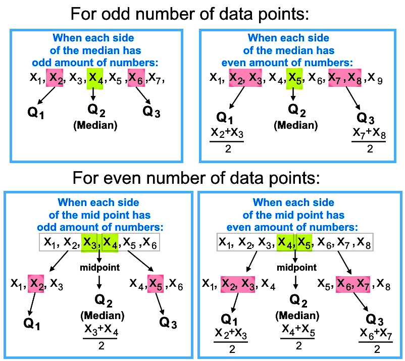
Therefore, the steps for finding quartiles are:
- Find the median of the data set.
- If the set has an odd number of values, then the median is the value in the middle and is equal to the second quartile.
- If the set has an even number of values, then the median is obtained by averaging the two middle values.
- If the set had an odd number of values, then the first and third quartile will be the median of the values before the middle value, and the median of the values after the middle value respectively.
- If the values before and after the middle value are an odd number of values, then their middle values will be the first and third quartiles.
- If the values before and after the middle value are an even number of values, then the median of each side is obtained by averaging the pair of middle values on each side. These will be the first and third quartile.
- If the set had an even number of values, the second quartile is calculated by averaging the two middle terms (obtaining the median of the set).
- Then, the set is divided by a midpoint. The whole first half is used to obtain the first quartile, and the whole second half is used to obtain the third quartile.
- If the values before and after the midpoint are an odd number of values, then their middle values will be the first and third quartiles.
- If the values before and after the midpoint are an even number of values, then the median of each side is obtained by averaging the pair of middle values on each side. These will be the first and third quartile.
The process has been summarized in the next diagram for each type of data you might found:

In summary, the measures of relative standing are those point marks or calculations that allow you to see where a particular data value is within the complete data set (or its proper distribution); the z-score will tell you how many standard deviations is a certain value away from the mean (either above or below it), the percentiles will tell you in which of the 99 points that divide the data set into 100 equal parts is your data point located and even provide you with a rank on how much data is above or below it, and the quartiles will do the same as the percentiles but dividing the data in four equal parts only.
Now, we recommend you to take a look at the next links so you can continue your independent studies in what you learned today. This lesson covers the most important measure of relative standing: the z-score, this short article contains an explanation of what is percentile rank and how is it different from percentage, and this page talks about other locations in a distribution, where they describe not only quartiles but deciles too! We suggest you to take a look to them so you can see more example problems.
This is it for the lesson of today, see you in the next one!
: z-score, a measure of how many standard deviations a data item is from the mean.
population:
sample:
z-score allows comparison of the variation in different populations/samples.
Quartiles: values that divide the data set into quarters.
bottom 25% of data
Median bottom 50% of data
bottom 75% of data
InterQuartile Range (IQR): represents the middle 50% of the data set.
Percentiles: indicates what percentage of the data falls below a certain value
Outliers: an outlier is a data point which lies an abnormal distance from all other data points.
Outliers are either,
a) above or b) below


