Understanding Continuous Random Variables and Normal Distribution

Dive into the world of continuous random variables and normal distribution. Master essential statistical concepts, from probability density functions to real-world applications in various fields.

Normal distribution and continuous random variables

Our lesson for today focuses on the topic of the normal probability distribution, and for that, let us have a review of what a probability distribution is, and the usage of continuous random variables on it, and then, jump into the normal distribution.

Probability distribution of a continuous random variable

A probability distribution is that which produces a graph where the vertical axis depicts the probability of a certain outcome during and experiment and not the frequency. In other words, a probability distribution is a depiction of a statistical experiment in which we are interested to know the probability for each possible outcome to occur, but not the precise outcomes from the experiment (depicted in frequency distributions).

Remember that probability refers to the chances of an outcome to occur in a random process.
When performing a random process, there are a variety of possible results (outcomes) from such experiment, but there is no way for the experimenter to know what each outcome from each trial will be; therefore, probability allows us make a guess of each possible outcome value based on the proportion of occurrence of each possible outcome in the set of all possible outcomes. Thus, probability provides the likelihood of a particular value to be the final outcome in a particular trial from the experiment.

The probability of a specific value of a random variable x to occur is mathematically defined as:

$probability \, = p(x) =$ $\large \frac{Number\;of\;successful\;outcomes}{Total\;number\;of\;possible\;outcomes}$
Therefore, we can see that a probability distribution is a tool that allows us to understand the values that a random variable may produce in a statistical experiment. But what is a random variable? And furthermore, how can it be continuous?
When recording the possible outcomes of a random experiment, each of the values produced as results throughout the experiment are what we call random variables. A random variable is formed by data points, each assuming a unique numerical value that has been produced through a trial, and which is a random result of our particular experiment; therefore, there is no way to know for sure what the result values of a random variable will be, but we can use its recorded outcomes and the probability of each to study the behaviour of a population.
For that, random variables are classified into two categories depending on the type of values they can contain: Discrete random variables and continuous random variables.

A discrete random variable is that which contains countable values: Whole numbers, integers. Therefore, discrete random variables refer to variables that deal with items that can be counted as complete units, not fractions or any infinitesimally small parts of a unit interval.
On the other hand, a continuous random variable may assume any value as long as it belongs to a particular defined interval that is being studied. Simply said, a continuous random variable can be any number within a specified interval, that includes decimal expressions or fractions; they are said to be continuous because they will contain every single value within the particular interval being studied, and so, no matter how small scale can you go within an interval, this variable is taking account of every single point within it.
For example, let us say a continuous random variable being studied by us may have values within 2 and 6, that means the variable can have an outcome equal to 3.2 or 5.23456 or 4.123 or even 2.0000000000000000001 because is still in between the values of 2 to 6!
If this same range was to be used for a discrete random variable, the possible values of such variable would only be the complete numbers: 2, 3, 4, 5, 6.

With the definition of the two types of random variables existen in statistics we can automatically understand that there will be two types of probability distributions: discrete and continuous, each of them making use of the type of random variable that gives them their name.

And so, a continuous probability distribution is the probability distribution of a continuous random variable; it describes a continuous interval of infinite possible outcomes and the probability of such to occur from all the possibilities within the continuous interval being studied. Since you can create tables and graphs with a probability distribution (just as can be done with the frequency distribution), a practical approach is to define a probability distribution as a list or graphic representation of all the possible values of a random variable and the probability of each of them occurring; thus, a probability distribution table lists the possible outcomes of the statistical experiment as classes and provides a value for the probability of each of these on the adjunct column; while a probability distribution graph can be done in the form of a histogram, or a curve.

A continuous probability distribution can also be though as a probability density function, where the area under the smooth curve of its graph is equal to 1 and the frequency of occurrence of values between any two points equals the total area under the curve between the two points on the x-axis. This is because there is an infinite amount of possible value outcomes in a continuous interval, which makes that the probability of each individual point on the interval to be an outcome goes to zero, therefore, the probability must be measured over interval pieces, and is equal to the proportion of area under the curve for that interval piece.

The most common types of continuous probability distributions are:

• The normal distribution
• The uniform probability distribution
• The exponential probability distribution

On this lesson we will focus on the first one.

What is a normal distribution?

A normal distribution, also called a Gaussian distribution, is the most common (and probably most important) type of continuous probability distribution that exists. Because of that, many academic texts and study materials may provide a normal distribution definition where they simply call them a continuous probability distribution.

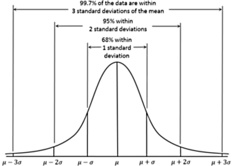
The normal distribution allows an statistician to work with the best approximation for a random variables behavior on real life scenarios as established in the central limit theorem : as long as the sample is sufficiently large, the shape of a random variables distribution will be nearly normal. The normal distribution curve looks like:



The main characteristics of a normal probability distribution are:

• It has a bell-shaped curve (reason why many times is simply called a bell curve).


• The normal curve is symmetric with the mean of the distribution as its symmetry axis and this mean has a value that is equal to the median and mode of the distribution (so, median = mode = mean in a normal distribution!).


• The total area under the bell curve (also called a Gaussian curve) is equal to 1, then half of it is on one side of the mean value (the axis of symmetry) and half is on the other side.


• The left and right tails on the normal distribution graph never touch the horizontal axis, they extend indefinitely because the distribution is asymptotic.


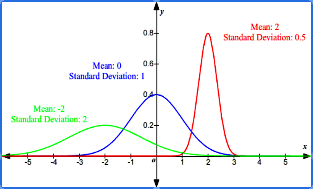
• The shape of the normal distribution and its position on the horizontal axis are determined by the standard deviation and the mean. The mean sets the center point, while the bigger the standard deviation, the wider the bell curve will be.

• About 68% of the population are within 1 standard deviation of the mean.


• About 95% of the population are within 2 standard deviations of the mean.


• About 99.7% of the population are within 3 standard deviations of the mean.

The standard normal curve

So far, we have found that the normal distribution is out best ally when studying real life large populations, but what happens if you study different variables from a same population? For that, we have the standard normal distribution.

A standard normal distribution (also called a z-distribution) is a normal distribution which has a value of zero as its mean and a value of one as its standard deviation. The values of any normal distribution can be translated into a standard normal distribution, meaning that any distribution can be re-scaled into a curve centered in the value of zero. This process is called standardization, and the resulting values corresponding to each point in the z-distribution are named z-scores. The formula to obtain such z-scores is:

$\large z = \frac{x\;-\;\mu}{\sigma}$
$\quad$Where:
$\quad z = z -$ score or standard score
$\quad x =$ original value from the normal distribution
$\quad\mu =$ mean of the original distribution
$\quad\sigma =$ standard deviation of original distribution

How is this useful? as we said before, if researchers are studying different characteristics from a population, all of these data distributions will have different means and standard deviations, making the comparison of the values throughout the different normal probability distributions very difficult.
Why? because you would need to use calculus (integration) to calculate the probability of each piece interval in each distribution for each set of data, where their scales are different. Even when data distributions come from the same population, the difference in their mean and standard deviation complicates such comparisons. Therefore, what we can do is to re-scale each distribution into a standard normal one and then compare them.


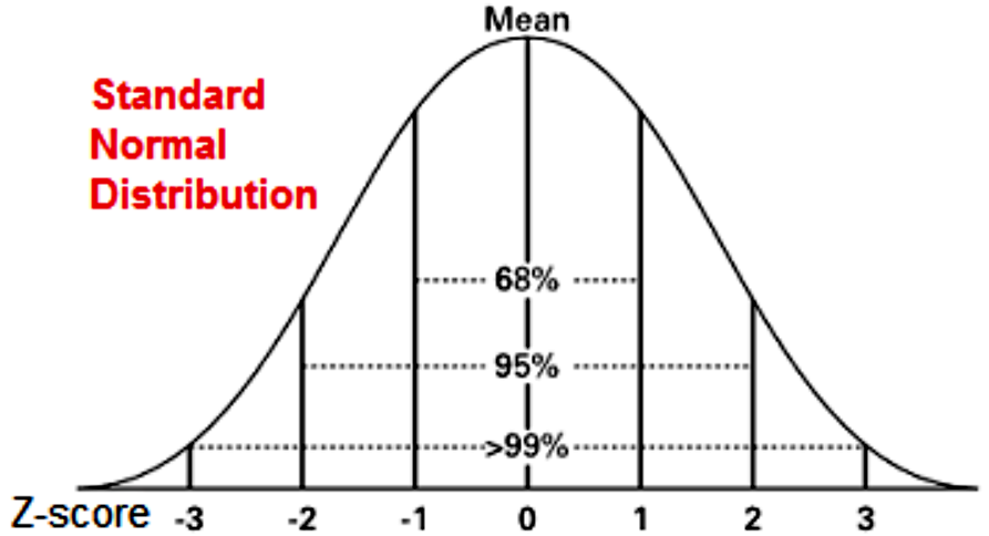
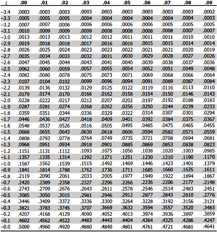
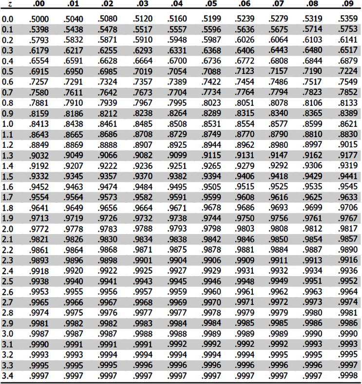
In simple words, statisticians made the practical decision to only calculate the probabilities of different values for one normal distribution: the z-distribution. With that, they created a standard normal distribution table (or z-table) with the standard scores and the probability of each. Then, you can use this as a standard to obtain the probabilities of intervals from any other normal distribution out there (you just need to translate the original normal distribution into the standard one and then check the z-table for probabilities).

As you can see, the standard normal distribution serves to estimate the probability of events from a normal distribution and to compare more than one of these distributions with one another; thus, allowing researchers of large populations to obtain a more complete picture of the population, and making the process faster and efficient.
Next we present the z-table for you to use it in our example problems in the next section:

Normal distribution examples

Example 1

Reading and using the Z Table, find the following:

1. the z-score when the area under the curve to the left of z is 0.3015.
2. The area from the mean to a z-score of 1.45.
3. The z-score when the area under the curve to the left of z is 0.7774.

Example 2

Finding Probabilities from Z-Scores
Answer the following questions based on the properties of standard normal distribution.

1. What is the probability of having a z-score that is less than 0.75?
2. What is the probability of having a z-score that is greater than -1.83?
3. What is the probability of having a z-score that is between -1.27 to 1.06?

Example 3

Finding Z-Scores from Areas
Answer the following questions based on the properties of standard normal distribution.

1. by Z table
2. by calculator

^***Notice that we will only include the method by the Z table, but you can watch our videos for this topic where you will find the calculation using the calculator explained.

1. Find the z-score that represents the bottom 70%.
2. Find the z-score that represent the top 70%.
3. Find the z-scores that represent the top 4% and the bottom 4%.

We have arrived to the end of our lesson.
Before you go, we recommend you to take a look at these materials on the normal (Gaussian) distribution. On our next lesson, we will finally talk about the relationship of the z-scores and random continuous variables, so stay tune and enjoy!