Mastering the Central Limit Theorem Formula

Unlock the power of statistical analysis with our comprehensive guide to the central limit theorem formula. Learn how to apply this fundamental concept to real-world data and enhance your math skills.

Central limit theorem

On this lesson we recall what the normal distribution is in order to use it as a basis for the study of data which is in high in volume.

What is the central limit theorem

The central limit theorem is a tool based on the idea that when you are studying a population, you can take different samples and calculate their means, then use such means to produce a distribution (which is called the sampling distribution of the mean) and this last distribution will be approximately a normal distribution as the size of the samples used to produce it increases.

Sounds complicated? Let us explain.

The central limit theorem is an important tool to obtain results coming from a large population, therefore, any time you work with the central limit theorem you should pay attention to two things given to you: the mean of the population and the standard deviation. Why? If you think about it, the issue when studying a large population is that you cant never really know the exact mean or standard deviation of it unless you talk with every single subject included in the population.
When doing statistical analysis of simulated populations this is possible, but in real life this is usually not a viable solution (imagine that you are studying the whole female population of Canada, it is highly unlikely you would be able to interview and get a direct response from every lady in the country). What do you do then? Take samples!

According to the central limit theorem, if you take every single possible sample of size n from a population, you would at some point reach all of the individuals in your population and thus obtain real values from the variable in question that is being studied from it. Again, as we mentioned before, this cannot be done (or at least, is highly unlikely). Therefore, the researchers could focus on taking as many samples as they can and as big as they can, to obtain information out of them.

The variables you need to know to understand the central limit theorem (sometimes just referred as CLT) are:

$\qquad \mu$ = population mean
$\qquad \sigma$ = population standard deviation
$\qquad n$ = sample size
$\qquad \overline{x}$ = sample mean
$\qquad \mu_{\overline{x}}$ = mean of the sample means
$\qquad \sigma_{\overline{x}}$ = standard deviation of the sample means

That being said, the central limit theorem assumptions can be summed up in the next quick sentence:

"The mean of a population is equal to the mean of the sample means"
Which translates into:

$\mu_{\overline{x}} = \mu \;$ and $\; \sigma_{\overline{x}}=$ $\large \frac{\sigma}{\sqrt{n}}$
In other words, when you have taken many equally sized samples of a population, you have calculated the mean of all of these samples (these are the sample means) and then you obtain the mean of these values, the result is the same as the mean of the entire population.
At the same time, if you graph the sample means, such graph will have an approximate normal distribution, no matter if the original data is not a normal distribution.
Furthermore, the greater the sample size, the closer the distribution of the sample means will be to a normal distribution and thus the better the central limit theorem approximation will be.
Because of this, the central limit theorem happens to be a tool that is used to obtain the level of accuracy of different statistics.

In other words, if we have equally large enough samples from a population we can use these to relate any data distribution (of any shape) from the original population to a normal distribution produced by the means of the sample means.

This is the most important characteristic of the central limit theorem! Not to actually do the sampling process, calculate the sample means and create the normal distribution itself, but the knowledge that resulting distribution will be a normal distribution! Simply said: you will not have to take the multiple samples, calculate their means and graph them into a distribution whenever you use the central limit theorem to solve statistical problems (this is usually done only when you are making the central limit theorem proof, which will be shown in the next section), but you will use the knowledge that this process produces a normal distribution (given that normal distributions are well understood in statistics) in order to obtain a good approximation of information related to any data distribution.

To finish with this section, once we want to work with actual numbers and the central limit theorem, we can obtain the standard scores of the values in the normal distribution of the sample means. Therefore, the central limit theorem formula for z-scores is equal to:

$\large Z= \frac{\overline{x}-\mu_{\overline{x}} } {\sigma_{\overline{x}}} = \frac{\overline{x} - \mu} {\frac{\sigma}{\sqrt{n}} }$
Where n is typically equal or bigger than 30.

Central limit theorem proof

To prove the statements from the central limit theorem lets see a simple example: Lets say you have gone to a school (where you have students from grade 1st to 12th), and you have made an announcement that anyone who loves pop music, please go to the auditorium after lunch. When you arrive to the auditorium after lunch, you have the following population of 560 students:


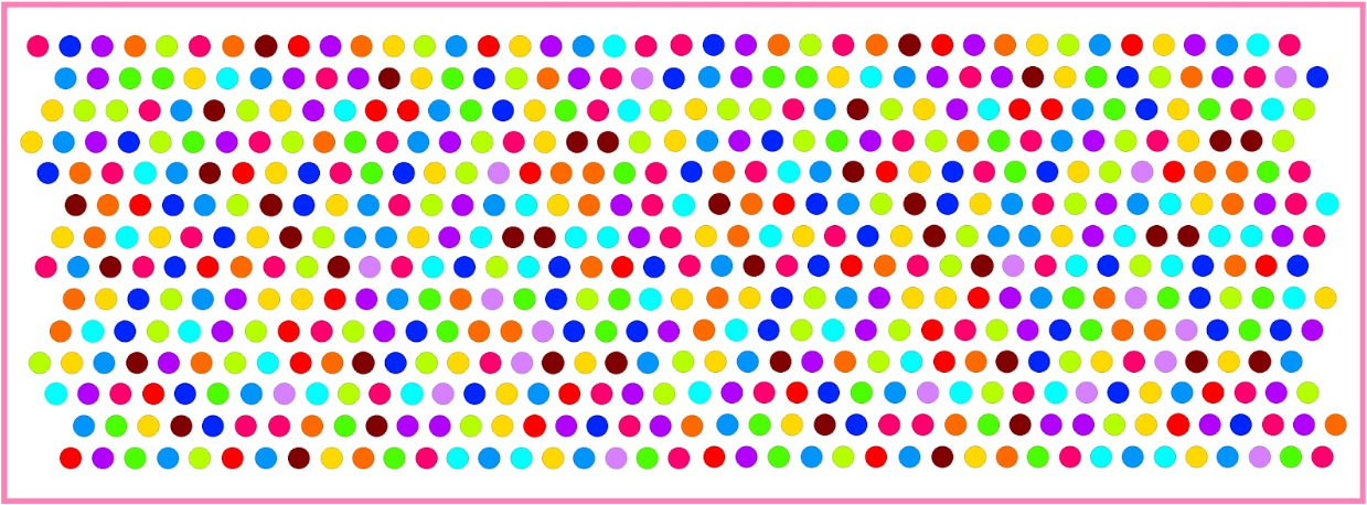
Where each color represents the grade in which students are in the following matter:


The distribution of such population has a mean of $\mu =6.673$ (which means that the average student is in grade 6th) and goes as follows:


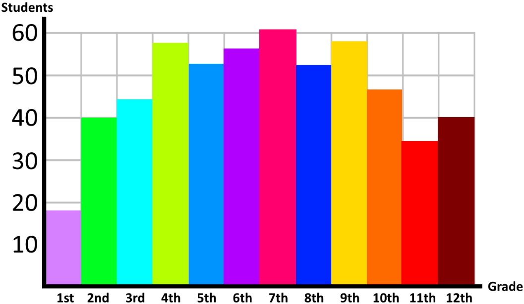
From such population we take 10 samples of size n=30, and we will use those to prove that when you obtain the mean of the sample means you will obtain an approximate normal distribution with them. So, our 15 equally sized samples are:


Calculating the mean of the sample means we obtain: $\mu_{\overline{x}}$ =6.446 which is pretty close to the mean of our population, and notice that if we were to draw the distribution of the sample means shown in figure 4, the distribution would look like a normal curve centered in the middle of grade 6th. How do we know that? Because all of the means of the samples fall into the grades 5th, 6th and 7th!

We wont be showing you the graph for it because we need many more samples to show the distribution with more detail, but we do recommend you to use a random number generator to create many samples and then calculate the mean of each to construct the distribution. You will see that an approximation to a normal distribution will come up and the mean of this distribution will be equal (or at least very similar, depending on how many samples you make) to the mean of the population.

Central limit theorem examples

On this section we will work on a central limit theorem example problem in which the method of obtaining the probability of an event is obtained thanks to standardization of a distribution (the method using z-scores), versus using the CLT. Then we will just apply the CLT in the second example.

Example 1
A population of cars has an average weight of 1350kg with a standard deviation of 200 kg. Assume that these weights are normally distributed.


For this question, we are looking for the area under the bell curve which contains values higher than the 1400kg mark in the original normal distribution, therefore, we need to find where this mark is in the standard normal distribution to then find the probability of the interval to the left of this mark using the Z-table and then subtracting this from 1. Using our equation for standard scores from our lesson on z-scores and continuous random variables we have that:

$Z=$$\large \frac{x\,- \mu}{\sigma}$
Where:
$\qquad z$ = $z$ - score or standard score
$\qquad x$ = original value from the original normal distribution
$\qquad \mu$ = mean of the original distribution
$\qquad \sigma$ = standard deviation of original distribution

Therefore, for this case we have: $x = 1400, \, \mu =1350 \;$and$\; \sigma = 200$.
Then:

$Z=$$\large \frac{x\,- \mu}{\sigma} = \frac{140 0\, - \, 1350}{200} = \frac{50}{200}$ $= 0.25$
The probability that a randomly selected car will weight more than 1400 kg is equal to the area under the curve of the standard normal distribution as shown below:


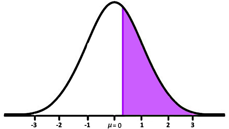
Therefore, the Z-value we have found so far is the mark on the x axis where the purple region above starts. Now, to find the probability value for the white region on the left side of the distribution above we use the Z-tables provided below:

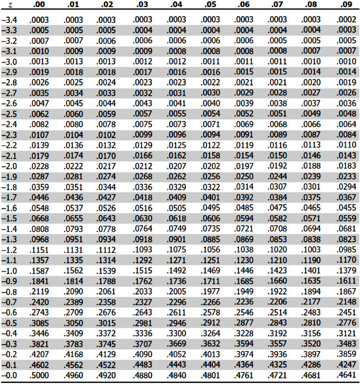
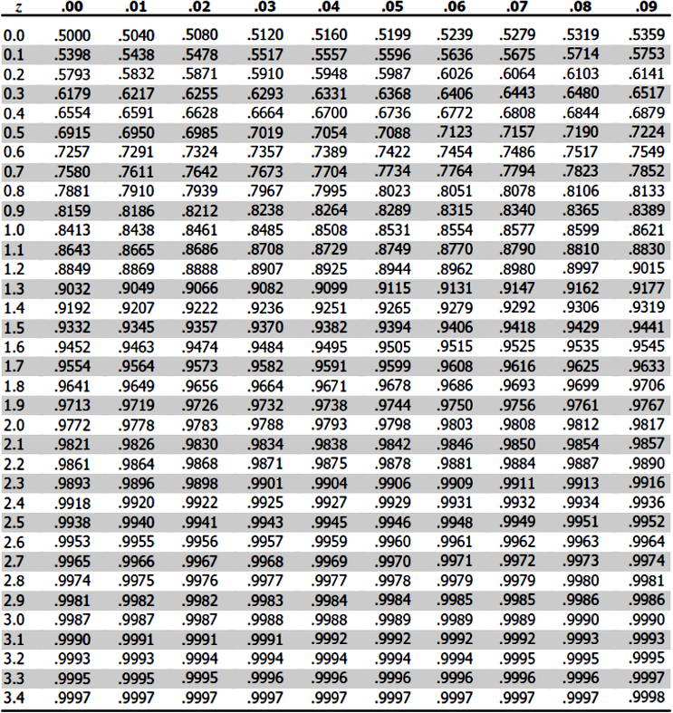
• For this case you will use the Z-table for a positive Z-value which is depicted in figure 7.
• Go to the row containing the first digit, and the first digit of the decimal point of your Z-value obtained in equation 2.
• Then go to the column containing the second digit after the decimal point of your Z-value from equation 2.
• Check where the row and column specified above intersect, this value is the probability of a car weighing less than 1400 kg.

Following the last steps, we know that the probability of randomly selecting a car that weighs more than 1400 kg is $P(x > 1400) = P(Z > 0.25) = 1 - 0.5987 = 0.4013.$
And this result is the area of the purple region shaded on figure 5.


For this case we want to find what is the probability that our sample mean is greater than 1400kg for a particular sample of 30 cars which is defined as: $P(\overline{x} > 1400)$
Notice that using the central limit equation as explained in equation 2, this is equivalent to:

$\large P(\overline{x} > 1400) = P(Z>\frac{1400 \,- \, \mu} {\frac{\sigma}{\sqrt{n}} }) = P(\frac{\overline{x} \, - \mu_{\overline{x}}} {\frac{\sigma}{\sqrt{n}}} > \frac{1400\, - \, \mu}{\frac{\sigma}{\sqrt{n}}} )$
We can solve the right hand side of equation 5 easily by plugging the values we already have: $\mu =1350 \;$and$\; \sigma =200 \;$and$\; n=30$ (since we are looking for the information on a group of 30 cars). Therefore:

$\large P(Z > \frac{1400\, - \, 1350}{\frac{200}{\sqrt{30}}} ) = P(Z > 1.37)$
This probability looks like:


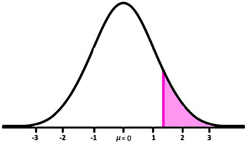
Using the z-table to find the probability up to $Z=1.37$:


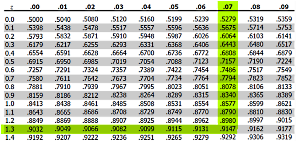
Therefore, $P(Z > 1.37) = 1 - 0.9147 = 0.0853$.

Example 2
Applying the Central Limit Theorem
Skis have an average weight of 11 lbs, with a standard deviation of 4 lbs. If a sample of 75 skis is tested, what is the probability that their average weight will be less than 10 lbs?

Following a similar process as the one described in the second part of our first problem, we have that:

$P(\overline{x} < 10 ) = P(Z< \frac{10\, - \, \mu}{\frac{\sigma}{\sqrt{n}}} )$
Since we have the following values: $\mu =11\,$and$\, \sigma = 4 \;$and$\; n=75$ (since our sample has 75 skis tested). Then:

$P(Z< \frac{10\, - \, 11}{\frac{4}{\sqrt{75}}} ) = P(Z < \,-2.165$
This probability looks like:


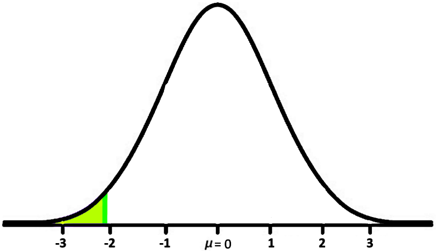
Using the z-table to find the probability up to $Z=-2.165$:


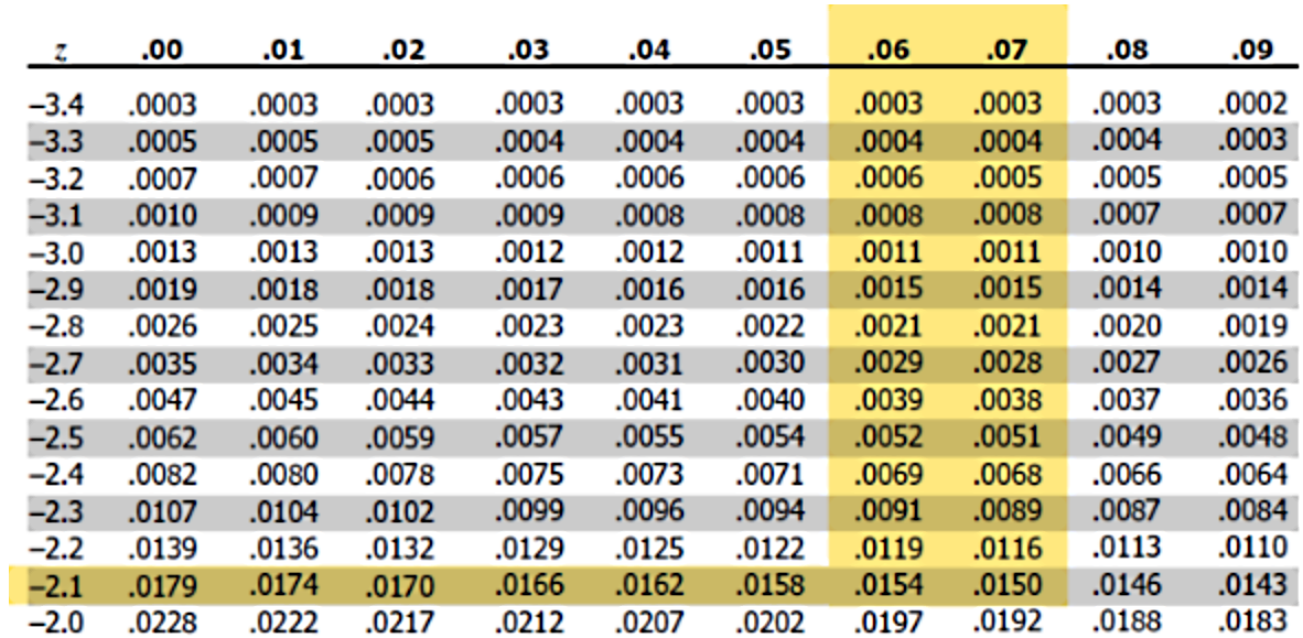
Therefore, $P(Z < -2.165) = 0.152$.

***
And so we have arrived to the end of this lesson.
We recommend you to take a look at this article on the central limit theorem to complement your studies.

This is it for today, see you on the next lesson!