Short Run Macroeconomic Equilibrium
The short-run macroeconomic equilibrium happens when
Where:
→ quantity of real GDP demanded
→ quantity of real GDP supplied in the short run
Graphically, this happens when the short-run aggregate supply and aggregate demand intersects
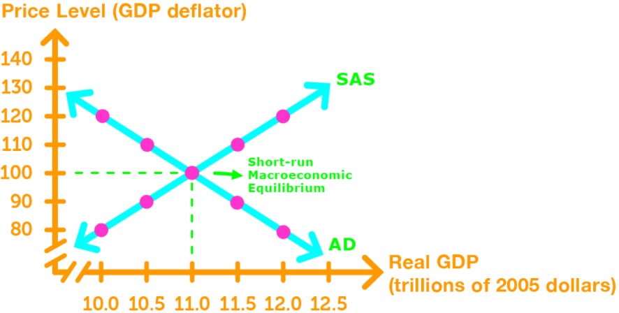
The intersection gives us the price level.
If the price level is not at the equilibrium, then there are two possible cases.
Case 1: The price level is above the short-run equilibrium price level.
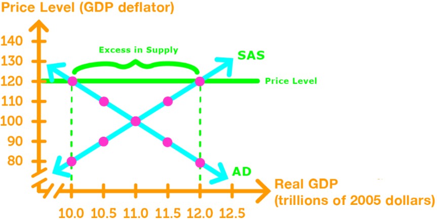
In this case, the firms are not able to sell all their outputs due to the excess in supply. Since remaining outputs get stockpiled, firms would eventually have to cut production until all their output is sold. Eventually, we go back to the equilibrium.
Case 2: The price level is below the short-run equilibrium price level.
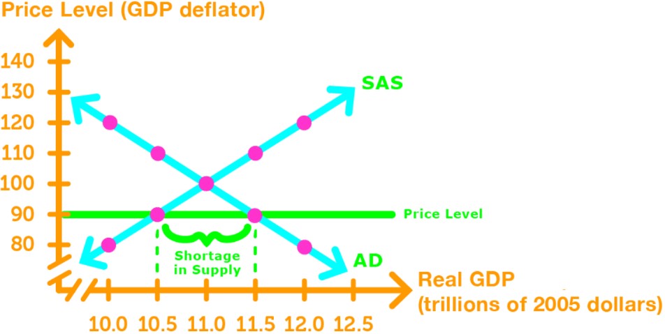
In this case, the firms are not able to meet the demand due to the shortage of outputs. The firms would have to increase production and costs to meet the demand of outputs they need. Eventually, we go back to the equilibrium.
Note: Recall that in the short run, money wage rate is fixed so it is possible that real GDP is greater or less than potential GDP.
Long Run Macroeconomic Equilibrium
The long-run macroeconomic equilibrium happens when potential GDP is equal to real GDP, and full employment is reached (unemployment rate = natural rate of unemployment). Equivalently, it happens when
Where:
→ quantity of real GDP demanded
→ quantity of real GDP supplied in the short run
→ quantity of real GDP supplied in the long run
Graphically, this is when the short-run aggregate supply, long-run aggregate supply, and aggregate demand all intersect.
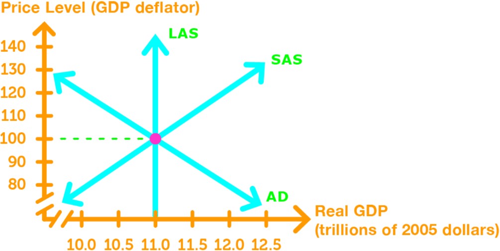
What if the price level is currently not at the long-run macroeconomic equilibrium? The idea is that eventually the price level will always go the long-run equilibrium price level.
Let’s look at 2 cases.
Case 1: The short-run equilibrium price level is above the long-run equilibrium price level.
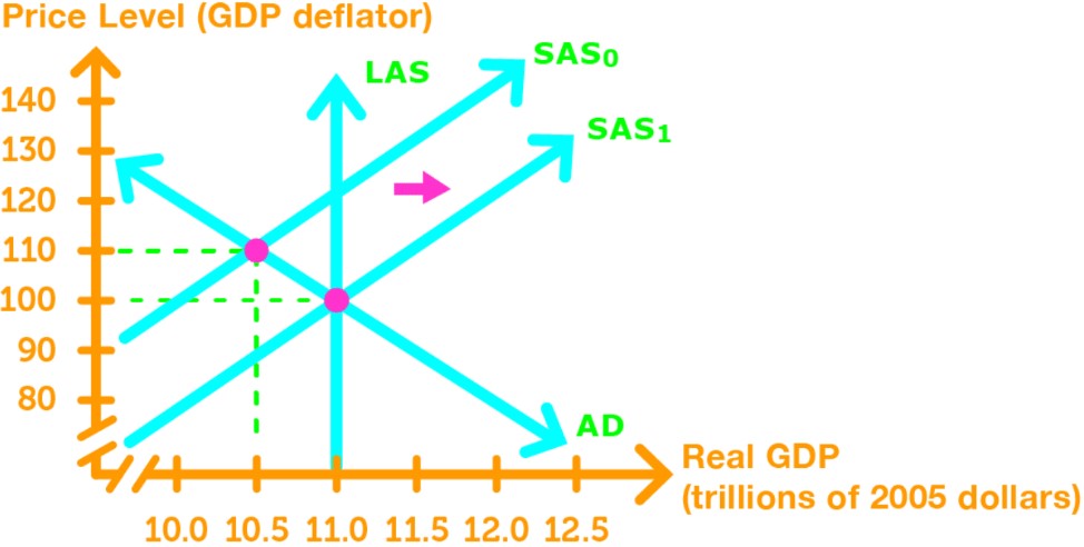
The money wage rate is very high, and unemployment rate > natural rate of unemployment. High money wage rate causes workers to supply more labor. So shifts right, becoming , and the price level is now at the long-run equilibrium price level.
Case 2: The short-run equilibrium price level is below the long-run equilibrium price level.
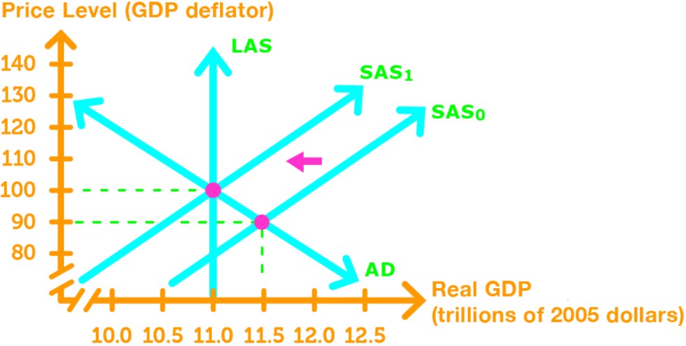
The money wage rate is very low, and unemployment rate < natural rate of unemployment. Low money wage rate causes workers to supply less labor. So shifts left, becoming , and the price level is now at the long-run equilibrium price level.
Economic Growth & Inflation with AS-AD Model
Economic Growth & Inflation: When potential GDP increases from labor productivity and growth of labor, the LAS curve shifts to right. Inflation in the economy causes the AD curve to shift to the right.
There are 3 types of ways the AD curve and LAS curve can shift.
Case 1: Inflation growth rate > GDP growth rate. So, the AD curve shifts more than the LAS curve, causing an increase in the price level.
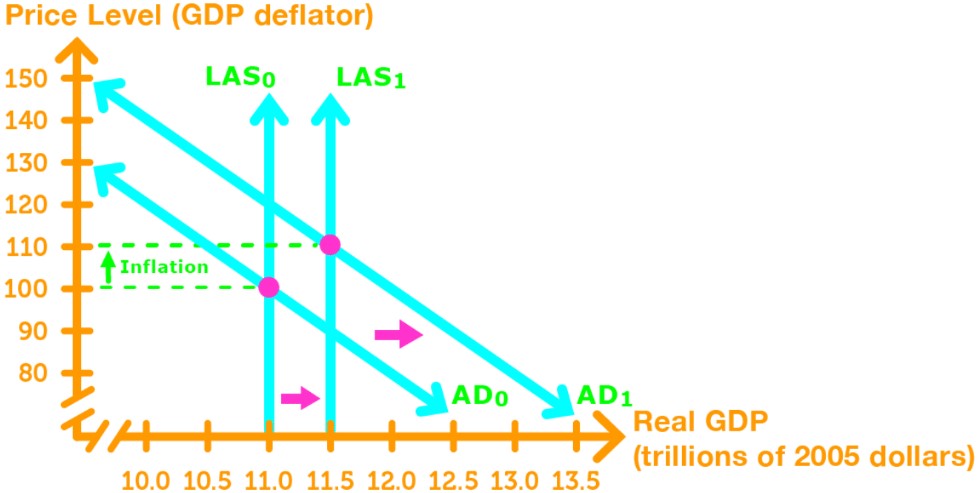
This results in an inflation to the price level.
Case 2: Inflation growth rate = GDP growth rate. So, the AD curve shifts the same amount as the LAS curve, causing neither an increase nor decrease to the price level.
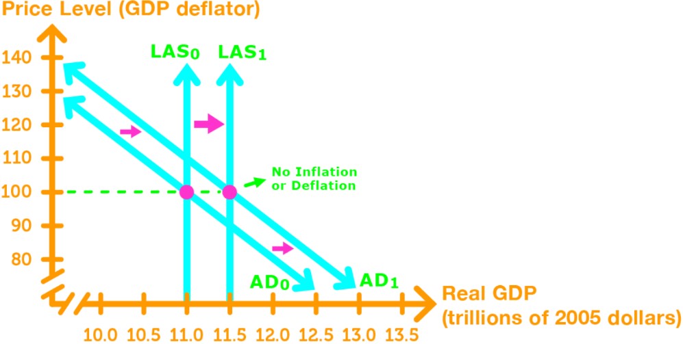
This results in no changes to the price level.
Case 3: Inflation growth rate < GDP growth rate. So, the AD curve shifts less than the LAS curve, causing a decrease in the price level.
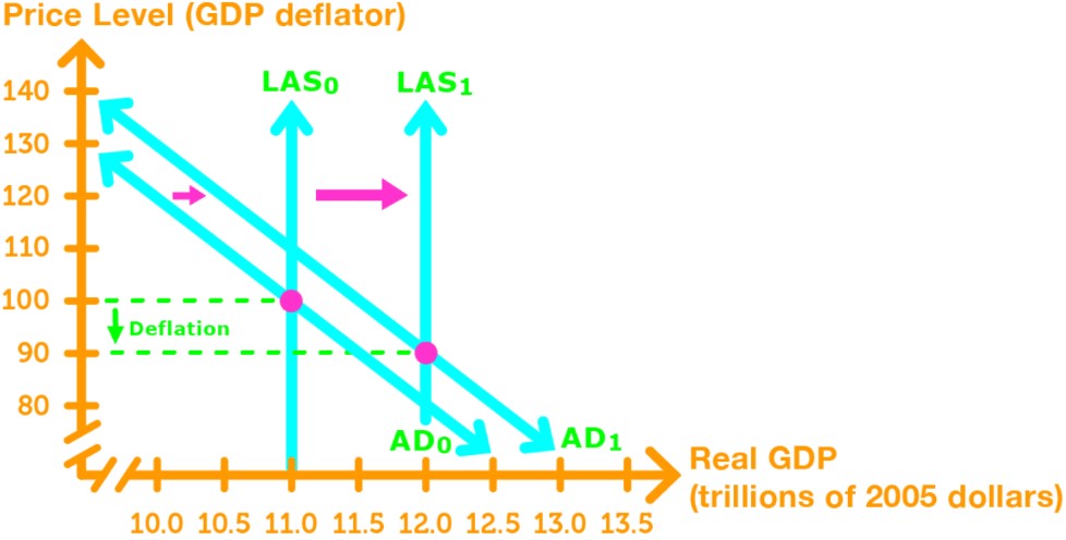
This results in a deflation to the price level.
Business Cycle with AS-AD Model
Recall that the output gap is the difference between real GDP and potential GDP. An output gap can either be inflationary or recessionary.
Case 1: When real GDP = potential GDP, there is an no output gap. The AS curve and AD curve intersects on the LAS curve.
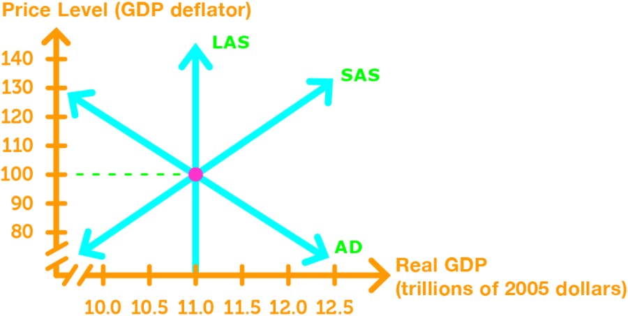
We achieve full-employment equilibrium (unemployment rate = natural rate of unemployment).
Case 2: When real GDP > potential GDP, there is an inflationary gap. The AS curve and AD curve intersects at the right of the LAS curve.
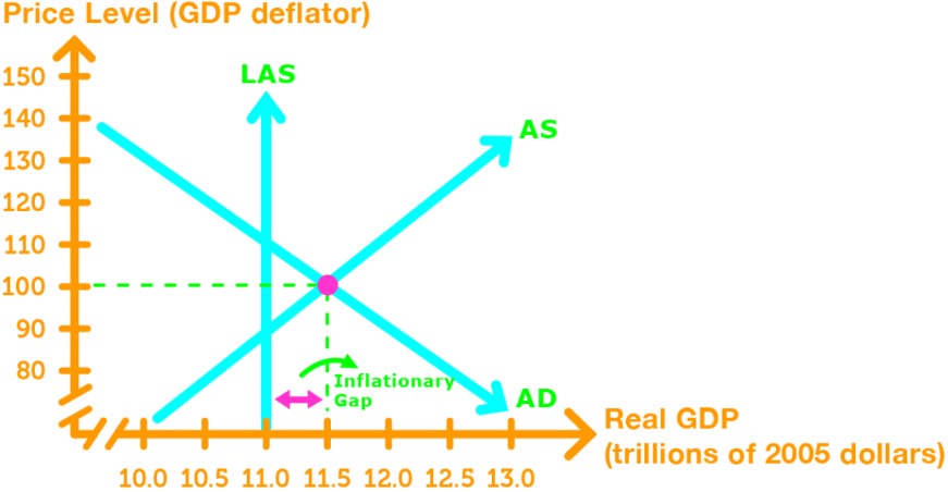
We achieve above full-employment equilibrium (unemployment rate < natural rate of unemployment).
Case 3: When real GDP < potential GDP, there is a recessionary gap. The AS curve and AD curve intersects at the left of the LAS curve.
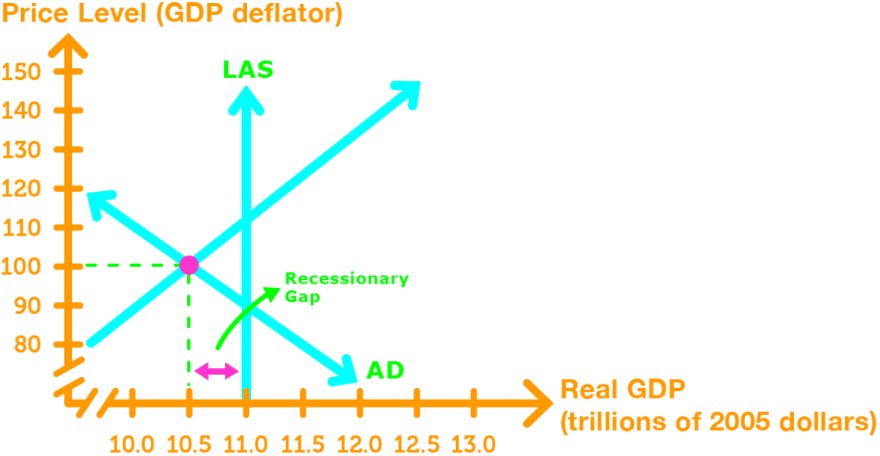
We achieve below full-employment equilibrium (unemployment rate > natural rate of unemployment).


