In this chapter, we are going to focus on the Keynesian model.
In this model, we look at aggregate expenditure, which is the sum of consumption expenditure, investment, government expenditure, and exports minus imports. We want to see how this is linked to real GDP.
Note: This section focuses mostly on the consumption expenditures
Consumption & Savings Function
There are a few factors that impact consumption expenditures and savings:
- Disposable income
- Real interest rate
- Wealth
- Expected future income
Disposable Income is equal to aggregate income subtracted by taxes and added by transfer payments.
In this section, we will keep real interest, wealth, and expected future income constant. By doing so, we can find the relationship between consumption expenditure and disposable income.
45° Line: is the line on the graph.
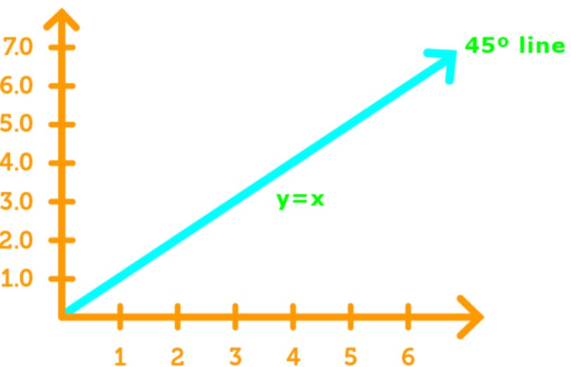
You will see this line when explaining other functions.
Consumption Function: is the relationship between consumption expenditures and disposable income.
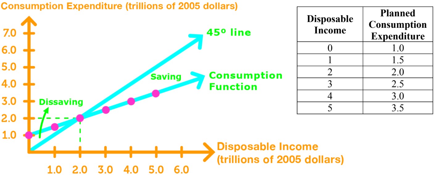
Notice from the graph:
- Function is a line that is upward sloping
- If the function is below the 45° line, then were saving
- If the function is above the 45° line, then were dissaving.
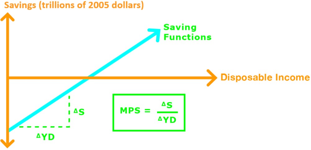
Saving Function: is the relationship between saving plans and disposable income.
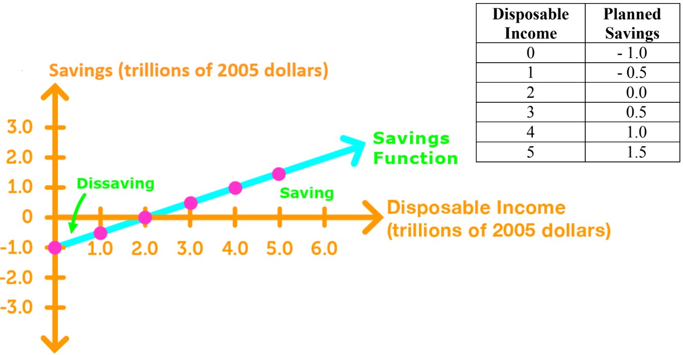
Notice from the graph:
- Function is a line that is upward sloping.
- If the function is above the -axis, then were saving
- If the function is below the -axis, then were dissaving.
Marginal Propensities
There are two marginal propensities we will be looking at
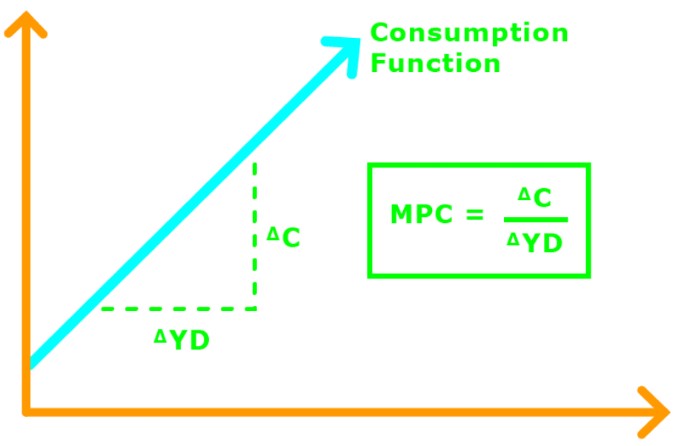
- Marginal Propensity to Consume (MPC): is the portion of the change in disposable income which will be used on consumption. To calculate this, we use the following formula
Where:
= change in consumption
= change in disposable income - Marginal Propensity to Save (MPS): is the portion of the change in disposable income which will be saved. To calculate this, we use the following formula
Where:
= change in savings
= change in disposable income
Property of Marginal Propensity: since disposable income is only used for either saving or consumption, then it must be true that
Dividing both sides of the equation by gives
Since we know that and , then
Applications of Marginal Propensities
Marginal propensities can be applied to a few things
- Consumption Function: the marginal propensity to consume is the slope of the consumption function.
- Saving Function: the marginal propensity to save is the slope of the savings function.
- Marginal Propensity to Import: is the portion of the change in real GDP that is spent on imports. To calculate this, we use the following formula
Where:
= change in imports
= change in income


