Students t-distribution
Continuing on our statistics course, in the lesson of today we will learn what is a t-distribution and how do we use it when constructing confidence intervals for the difference between two population means, but before we continue onto the full explanation of the topic, we need to get a little review on what is a normal probability distribution, and then how do we make a standard normal distribution, so that we can compare our concepts and their usage to perform similar statistical tests.
A little review on Normal Distributions
A normal distribution, also called a Gaussian distribution, is the most common (and probably most important) type of continuous probability distribution that exists. Because of that, many academic texts and study materials may provide a normal distribution definition where they simply call them a continuous probability distribution.
The normal distribution allows a statistician to work with the best approximation for a random variables behavior on real life scenarios as established in the central limit theorem : as long as the sample is sufficiently large, the shape of a random variables distribution will be nearly normal. The normal distribution curve looks like:
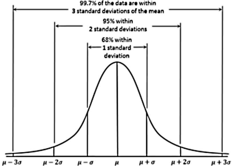
The main characteristics of a normal probability distribution are:
- It has a bell-shaped curve (the reason why many times is simply called a bell curve).
- The normal curve is symmetric with the mean of the distribution as its symmetry axis and this mean has a value that is equal to the median and mode of the distribution (so, median = mode = mean in a normal distribution!).
- The total area under the bell curve (also called a Gaussian curve) is equal to 1, then half of it is on one side of the mean value (the axis of symmetry) and half is on the other side.
- The left and right tails on the normal distribution graph never touch the horizontal axis, they extend indefinitely because the distribution is asymptotic.
- The shape of the normal distribution and its position on the horizontal axis are determined by the standard deviation and the mean. The mean sets the center point, while the bigger the standard deviation, the wider the bell curve will be.
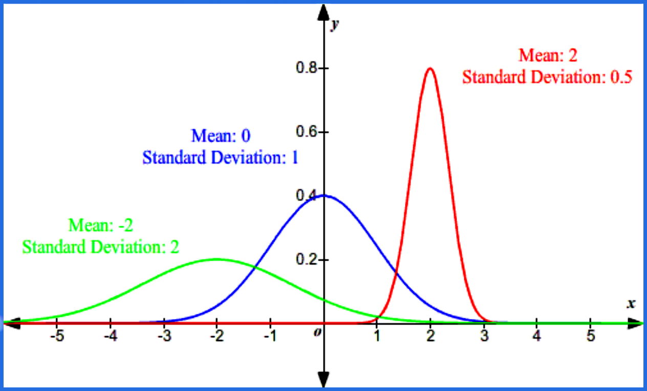
Then we have the standard normal distribution, also called a z-distribution, is a normal distribution which has a value of zero as its mean and it runs along its horizontal axis in units of its standard deviation. The values of any normal distribution can be translated into a standard normal distribution, meaning that a normal distribution can be re-scaled into a curve centered in the value of zero. This process is called standardization, and the resulting values corresponding to each point in the z-distribution are named z-scores.
What is a t distribution
What is the t distribution in statistics? The Students t-distribution is a continuous probability distribution that comes up when our data sample is considerably small and we do not know its variance because the standard deviation is unknown.
The t distribution is a probability distribution similar to the standard normal distribution, but this one can be done without knowing the standard deviation of the population. When comparing the normal distribution versus t distribution, we see that the graph t distribution has tails which are bigger or fatter'' than the standard normal distribution, which means that there is a higher probability of finding a data point in one of the tails than when working with a normal distribution. That is one reason t-distribution graphs look shorter than the normal distribution, because more of its area is gone to the tails.
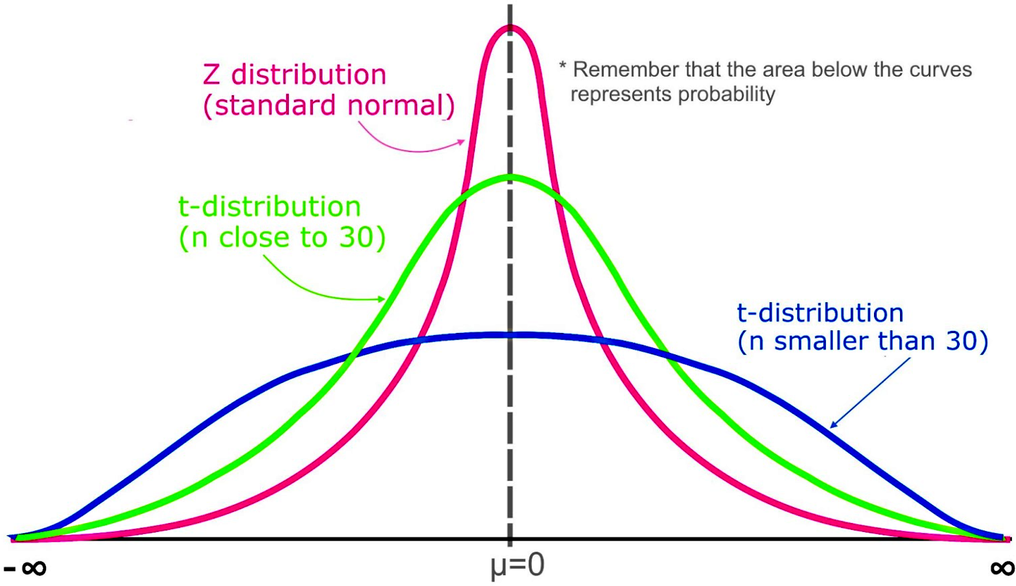
Remember that the area under a t-distribution and z-distribution curve represents probability, the total area in each curve is equal to 1. And so, this means the probabilities are similarly but still differently distributed in each of these probabilities.
The reason for a t chart distribution shape comes from the fact that t-distributions are used for smaller samples. When studying characteristics of a population, there are different sampling methods that need to be followed in order for the sample to be representative of a population. It has been found that when data points are graphed in a probability distribution, the bigger the sample the more data points will be found to be close or equal to the mean, and so a smaller sample size provides a higher proportion of the sample to be spread out.
And so, what are t distributions when graphed? They are still bell shaped distributions but since your sample is smaller, one single individual point being far away from the mean is a bigger proportion of the total sample than when your sample contains many more individual points, and so this characteristic makes its tails thicker.
Derivation of the t distribution
In order to find the t distribution values for a specific problem setting we use the significance level and the degrees of freedom for the case to locate the specific t-score dividing the region of rejection and failure-to-reject. We do this by finding the intersection point of the degrees of freedom and the significance level in a Students t distribution table.
Notice, these values are actually critical values for a t distribution graph (locations in the horizontal axis of the graph that provide a division among different regions, specifically the zone denoting the rejection of the null hypothesis and the zone denoting the failure to reject it).
An example of these t distribution tables is given in the section for the step-by-step instructions to solve a hypothesis test for a population mean.
Besides the tables, we can calculate the test statistic t-score using the following formula:
= Student t-distribution
= the sample size
= the population mean
= the sample mean
= the sample standard deviation
When to use t distribution
In the previous lesson we discovered how to make a confidence interval for estimating a population mean. However we knew what the population standard deviation () was. However it is not always the case that is known.
When building a confidence interval, remember that we use the formula:
Where the margin of error is defined as:
If the population standard deviation () is unknown then to make a confidence interval to estimate the population mean we cannot use our old formula for error as it requires a knowledge of . So instead we are required to use a thing called t-scores ().
Stop for a moment and check the notation for the t-scores:
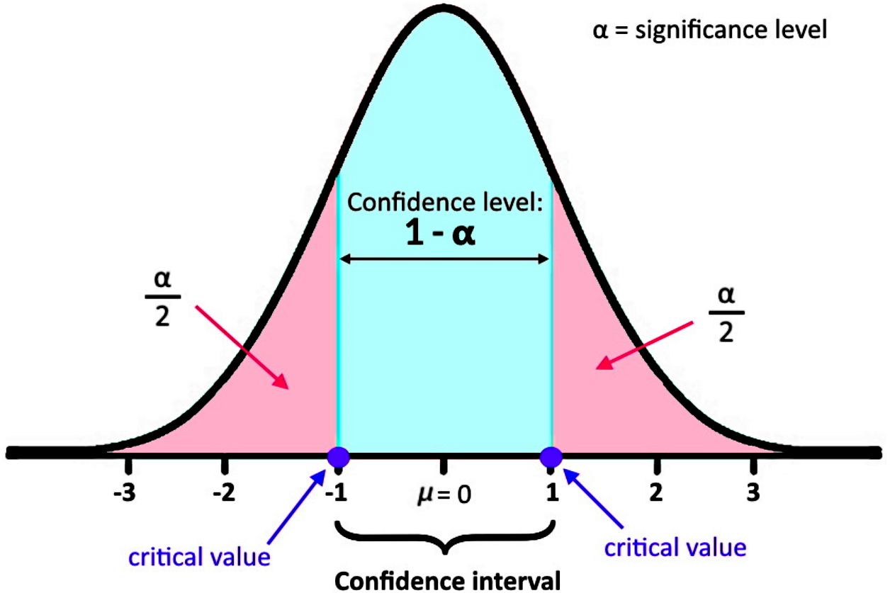
The comes from the Students t distribution and the subindex comes from the significance level () and how it is spread in the tails of the distribution. Remember that the significance level can be located either on the right or the left tail of a distribution. When the significance level is divided by two, it means half of it is found on the left tail and the other half on the right tail of the distribution as shown below:
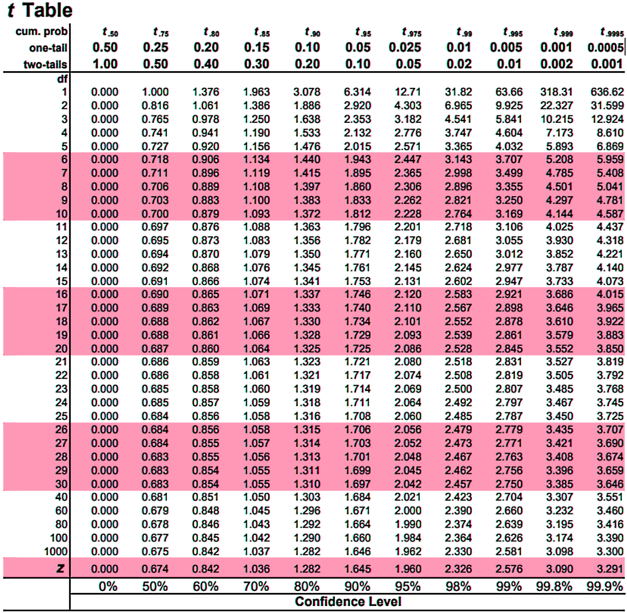
To find the t-scores we need the value of the significance level, the amount of degrees of freedom for the specific Student t distribution and a full t distribution table such as the one shown below:
The degrees of freedom are obtained by subtracting the sample size minus 1:
And you may be wondering how to use a students t distribution table, well it is easy!
Notice the top row shows the value of the significance level and it differentiates between a one tail or two tailed case, while the left column contains the number of degrees of freedom. The only thing you need to do is look for the row of degrees of freedom you have, and the column of the significance level you have, and where the row and column meet, that is the value of your t-score!
If you still have any question on how to read a students t distribution table just take a look at example problem 2 (part a) below, where it is explained step by step.
Once we find the t-scores for particular values (this is done in a similar way to finding z-scores) we have a new formula for the Margin of Error:
Find a t distribution example problems
Example 1
Determining a Confidence Interval for a Population Mean using t-distributionsThe "Vendee Globe" is an around the world solo yacht race. In a particular year 31 sailors did the race and finished with an average time of 123 days, with a standard deviation of 11 days. With a t-score of = 2.45 construct a confidence interval for the average amount of time it takes the average Vendee Globe sailor to circumnavigate the world (sail around the world).
We have the following information for this problem:
= 31 = Sample size
= 11 days = Sample standard deviation
= 123 days = sample mean
= 2.45 = t score
In order to find the confidence interval we take a look at the population mean and the values possible below and above it. We set this up easily because we know we will have values spreading out from the mean in the following manner:
Where:
= sample mean = 123 days
= margin of error
= population mean
Using the formula for error, we calculate the left hand side and right hand side of the mean definition:
And so the confidence interval is as follows:
Therefore, the Vendee Globe sailors take in between 118.16 to 127.84 days on average to circumnavigate the world.
Example 2
In "Anchiles", a small made-up town near the equator, 15 random days were sampled and found to have an average temperature of 28°C, with a standard deviation of 4°C. Assume that the average daily temperature of this town is normally distributed.a. With a 95% confidence where does the average daily temperature of Anchiles lie?
We have the following information for this problem:
= 15 = Sample size
= 4 °C = Sample standard deviation
= 28 °C = sample mean
Where the margin of error is:
To calculate this, we need to obtain the t-score. Remember that we can obtain a t-score from a t-table of values using the significance level () and the degrees of freedom in t distribution for this case.
The significance level can be easily obtained from the confidence level of 95%, which means that:
The degrees of freedom are calculated from the subtraction:
And with this information we use the t table to find the t-value:
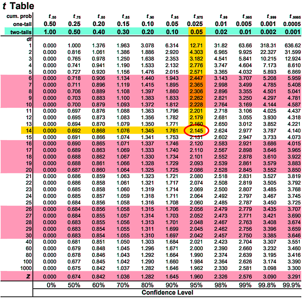
Notice that we used the two-tail significance level value because when looking for the t-score at this time, we are looking for where refers to a significance level (rejection area) divided in two equal parts which belong to the tails of the distribution curve.
And so, using the t-value found of = 2.145 we can calculate the error value for this problem:
And finally find the confidence interval of the average daily temperatures:
And so we can say with 95% of confidence that the daily average temperature of Anchiles falls somewhere between 25.785°C and 30.215°C.
b. What if we knew that in fact the standard deviation of temperature was 4°C for the entire population? Then with a 95% confidence where does the average daily temperature of Anchiles lie?
For this question we actually have the population standard deviation so we can use z-scores instead of t scores!, let us gather all of the information we have:
= 15 = Sample size
= 4 °C = population standard deviation
= 28 °C = sample mean
1 - = 95% = 0.95
= 0.05
And we are looking for the confidence interval
Where:
In order to calculate the error we need to find the z-score , notice this one comes from a two tailed test. Since the confidence level is 95%, that means that in order to find the point on the horizontal axis of the distribution for the right tail we add the surfaces of the confidence level (0.95) and the area on the left tail (0.025)... and so you have an area of 0.975 to use in the z-table to find the value of the z-score:
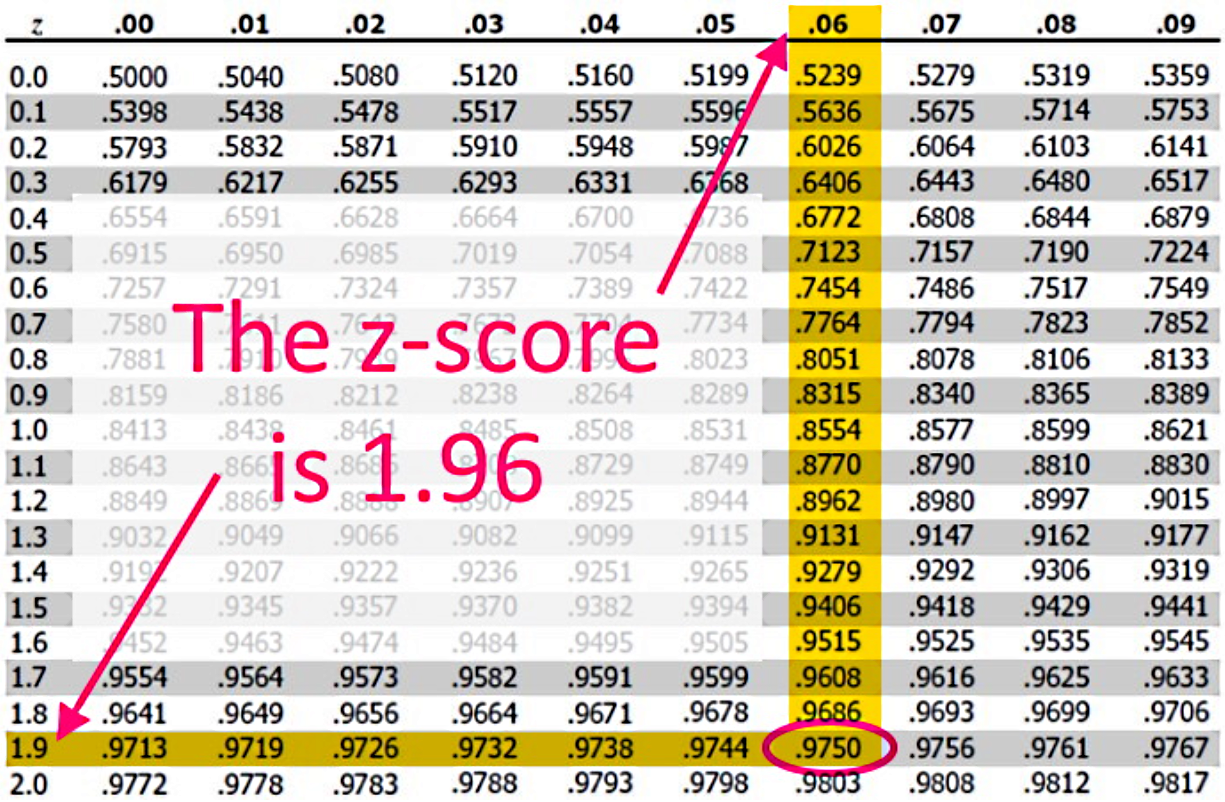
And so:
Finally find the confidence interval of the average daily temperatures:
Therefore the average daily temperature of Anchiles lies between 25.9757 to 30.0243 degrees celsius.
c. From the previous two questions, which has a larger confidence interval? Why might that be the case? Look at the t-scores as the sample gets larger and larger.
The first case has the largest confidence interval, take a look at our video lesson so you can see the graphic description of how the size of the sample does affect t-scores.
The first case has the largest confidence interval, take a look at our video lesson so you can see the graphic description of how the size of the sample does affect t-scores.
Example 3
Determining the Sample Standard Deviation with a given Margin of ErrorFrom a sample of 25 new drivers it was found that the average age that a young adult in British Columbia receives their driver's license is given with a 90% confidence as somewhere in the interval of 16.72 < < 23.28 years old. Assume that the age that new drivers receive their license is normally distributed. What was the standard deviation from this sample?
Since we are looking for a sample standard deviation, we know that we need to use the formulas for a Students t distribution to find the value of s. But first, we need to gather all the information for the problem:
= 25 = Sample size
1 - = 90% = 0.90 = confidence level
= 0.10 = significance level
16.72 < < 23.28 years old = confidence interval
Using the formula for the confidence interval we have that:
Solving the system of equations:
So the error is equal to 3.28 and the sample standard deviation is 20.
Now we use the equation for the error to solve for the sample standard deviation:
For this we need the t-score , and it comes from a two tailed test.
To find the t-score we need the t-distribution degrees of freedom which can be found by doing the subtraction: - 1 = 25 - 1 = 24. And we also need the confidence level which is equal to 0.10.
With that, we use a Students t-distribution table:
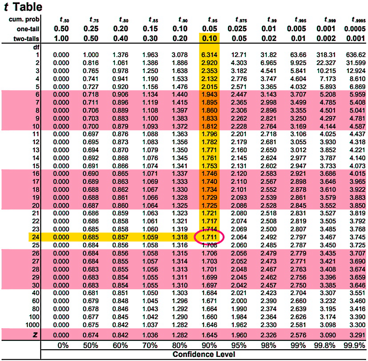
And so:
Therefore the sample standard deviation is 9.585 years.
To continue working on examples of building confidence intervals using a t-distribution we recommend you to take a look at the following t distribution calculator where you can find t-scores faster. Practice at home finding values for t-scores using the t distribution table and checking them with the calculator.
In the previous section we discovered how to make a confidence interval for estimating population mean. However we knew what the population standard deviation () was. However it is not always the case that is known.
If population standard deviation () is unknown then to make a confidence interval to estimate population mean we cannot our old formula for error: as it requires a knowledge of . So instead we are required to use a thing called t-scores (.
Once we find the t-scores for particular values (this is done in a similar way to finding z-scores) we have a new formula for the Margin of Error:


