Confidence intervals to estimate population mean
What is a confidence interval
A very simple confidence interval definition can be provided by referencing to the empirical rule above (figure 1) since it is clear that such interval must be the range of values comprising a particular confidence level. This is simple to remember since we can define interval simply as a range of values of a particular parameter, then for the case of a confidence interval, we can just add that this particular range of values is the one that is believed to contain a specific parameter mark of the population that is being studied, in other words, is the range in which a confidence level falls (and thus why it is likely that a particular parameter value will fall in there).
Confusing? Just take a look at the figure below:
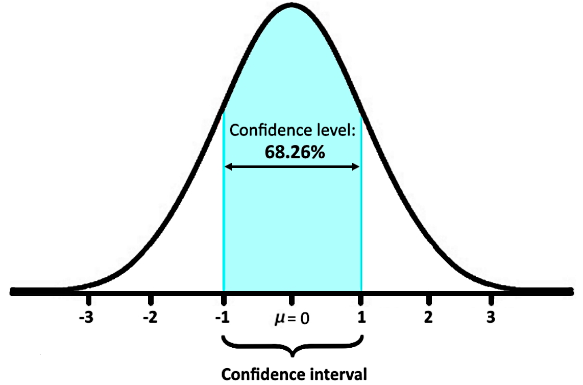
The percentages of 68.26%, 95.44% and 99.72% showcased in the normal distribution from figure 1 represent confidence levels, and belong to what we call two-sided confidence intervals because their range starts and ends within the distribution. Just take a look at figure 2, you can see that the confidence interval has a lower limit (-1) and an upper limit (1).
Mathematically speaking, a confidence interval is given by:
or equivalently:
Where:
= the critical value
= the point estimate, a sample estimate.
= the population proportion (this is the data we are concerned with ultimately finding)
= sample size
All this being said, for this lesson you will need the next important concepts:
The confidence interval is the plus-or-minus figure usually reported in newspaper or television opinion poll results. For example, if you use a confidence interval of 4 and 47% percent of your sample picks an answer you can be sure that if you had asked the question of the entire relevant population between 43% (47-4) and 51% (47+4) would have picked that answer.
The confidence level tells you how sure you can be. It is expressed as a percentage and represents how often the true percentage of the population who would pick an answer lies within the confidence interval. The 95% confidence level means you can be 95% certain; the 99% confidence level means you can be 99% certain. Most researchers use the 95% confidence level.
When you put the confidence level and the confidence interval together, you can say that you are 95% sure that the true percentage of the population is between 43% and 51%.
The wider the confidence interval you are willing to accept, the more certain you can be that the whole population answers would be within that range. For example, if you asked a sample of 1000 people in a city which brand of cola they preferred, and 60% said Brand A, you can be very certain that between 40 and 80% of all the people in the city actually do prefer that brand, but you cannot be so sure that between 59 and 61% of the people in the city prefer the brand.
Factors that Affect Confidence Intervals
There are three factors that determine the size of the confidence interval for a given confidence level. These are: sample size, percentage and population size.
Sample Size
The larger your sample, the more sure you can be that their answers truly reflect the population. This indicates that for a given confidence level, the larger your sample size, the smaller your confidence interval. However, the relationship is not linear (i.e., doubling the sample size does not halve the confidence interval).
Percentage
Your accuracy also depends on the percentage of your sample that picks a particular answer. If 99% of your sample said Yes and 1% said No the chances of error are remote, irrespective of sample size. However, if the percentages are 51% and 49% the chances of error are much greater. It is easier to be sure of extreme answers than of middle-of-the-road ones. When determining the sample size needed for a given level of accuracy you must use the worst case percentage (50%). You should also use this percentage if you want to determine a general level of accuracy for a sample you already have. To determine the confidence interval for a specific answer your sample has given, you can use the percentage picking that answer and get a smaller interval.
Population Size
How many people are there in the group your sample represents? This may be the number of people in a city you are studying, the number of people who buy new cars, etc. Often you may not know the exact population size. This is not a problem. The mathematics of probability proves the size of the population is irrelevant, unless the size of the sample exceeds a few percent of the total population you are examining. This means that a sample of 500 people is equally useful in examining the opinions of a state of 15,000,000 as it would a city of 100,000. For this reason, the sample calculator ignores the population size when it is large or unknown. Population size is only likely to be a factor when you work with a relatively small and known group of people.
In general, the critical value definition refers to a particular point on the horizontal axis of a graph which divides the area of the graph in two pieces (not necessarily equal pieces). On this case we will focus on critical values of z (also called z critical values), which means that we will be looking at critical values related to a z-score and thus our graph will always be a standard normal distribution (z-distribution).
A critical value of z allows you to divide the area under the standard normal curve into two pieces, and thus, it can help you in the calculation of probabilities or any other related characteristics of the data points from the distribution.
When using confidence intervals delimiting the area under the standard normal curve for a confidence level, we can use any of the edges of the interval as a critical value and either calculate the probability and confidence level being delimited by the interval; or, if the confidence level is given, we can find the critical value by looking at the z-score which produces the areas delimited by the interval.
How does this work? Let us explain:
Think on the empirical rule shown in figure 1. In this case, you can see that there is a confidence level of 0.6826 that a data point from this set will be located inside the confidence interval delimited by the cyan area under the curve. For this case, we know that the edges of this confidence interval are -1 and 1, but if only the percentage of 68.26% had been given to you, how would you know?
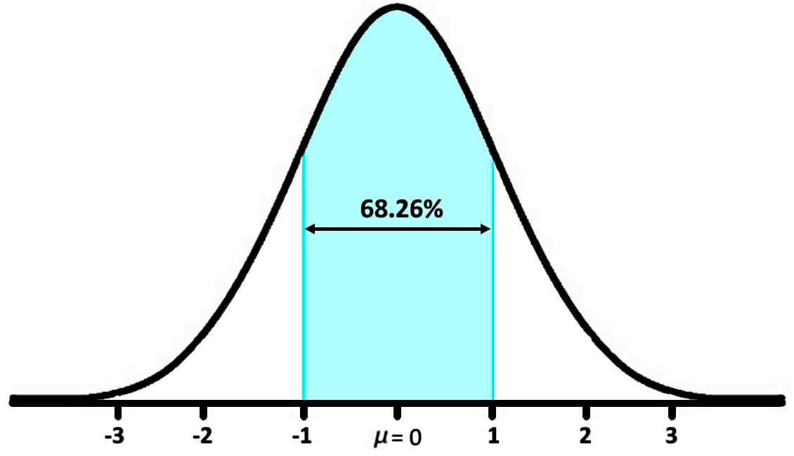
Well, if the confidence level in cyan color occupies 68.26% of the total area under the curve (which is 1) it means that it covers an area of 0.6826, leaving 0.3174 of the area divided in two pieces, one on each side.
Therefore, the tail area on the left would be half the 0.3174, and the tail area on the right would be the other half. Each of them would have a value of 0.1587. To find the critical value, we look at the tail area on the left and see that this 0.1587 is equivalent to the probability of a data point to be located on this area, which is delimited by a certain z-score (or z-value).
To obtain this z-value we just had to go and take a look at the z-tables and find the z-score which produces the probability value of 0.1587. So you can think of the z-table as a table of critical values if you know how to use it! The z-tables are below for you to take a look.
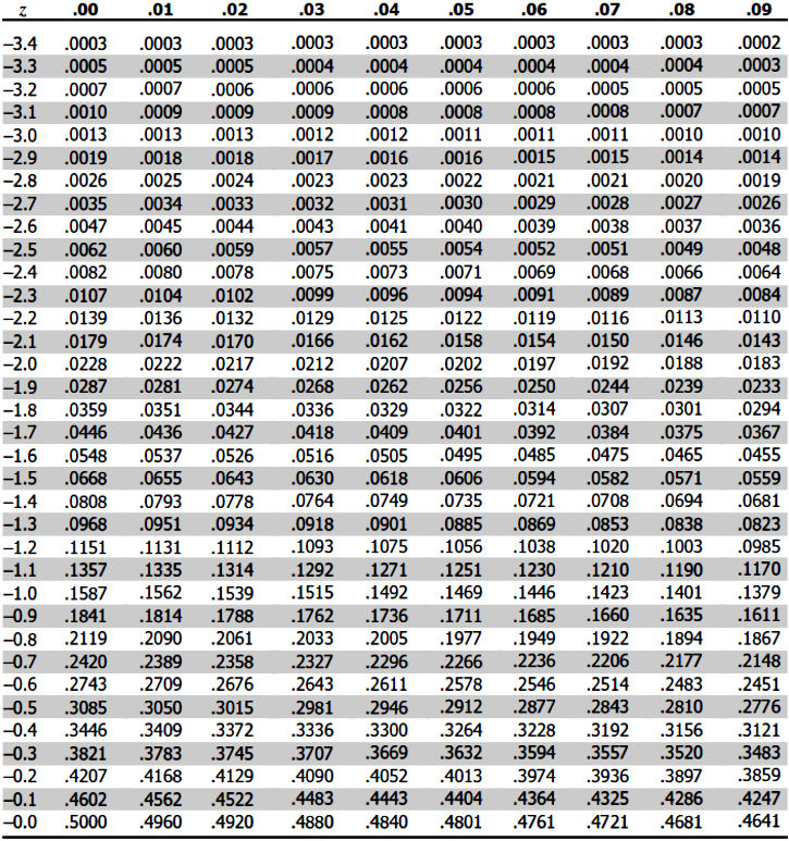
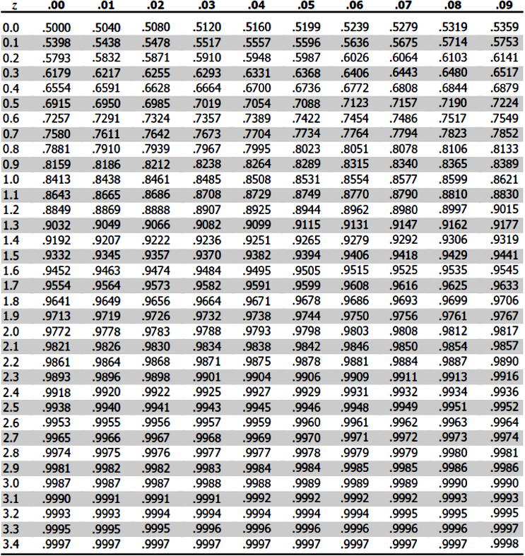
As you can see, the z-score which produces a probability value of 0.1587 is , which is correct! This is the critical value for a two sided confidence interval with a confidence level of 0.6826. Or in other words, that is the value on the horizontal axis where the confidence interval starts.
We know if correct, because we already knew this from the empirical rule. You think this example was redundant? Then let us take a look at the next section of our lesson, where the first example problem will ask you to find the critical values in this same way we just did above, but now, for distinct and varied confidence levels.
How to find a critical value
The steps to find a critical value when knowing the confidence level are:
- Draw the standard normal curve with the proper confidence level being portrayed.
- Identify the limit (or limits) of the confidence interval.
- If the confidence interval belongs to the left-most side of the distribution, then use the area proportion of the confidence level to find the corresponding z-value on the z-table.
- This is your critical value.
- If you are looking at a two-sided confidence level centered at the mean, then you need to calculate the area under the standard normal curve which doesnt belong to the confidence level (this area is called ).
- You will have half of on the left, and half of it on the right.
- Calculate the value of /2 and then use this value to find the corresponding z-value from the z-table. Notice this is done, since this /2 value is equal to the area under the curve on the left tail of the distribution
- This is your critical value (the value of z at which the confidence interval has its lower limit).
As you can see, critical values and confidence levels are strongly related to each other when studying probabilities in the standard normal curve. Also notice, at this point we dont have to calculate critical values, is more like finding critical values using the z-tables.
How to find a confidence interval?
In order to have a better idea on how to calculate a confidence interval, let us take a look at the next problem examples:
Example 1
Determining a Confidence Interval for a Population Mean At a wrecking yard 40 cars are weighed and found to have an average weight of 1500 lbs. The standard deviation of the weight of all cars is 175lbs. With a critical value ofWhat is the confidence interval for the weight of all cars?
On this case, the data is:
Where:
1500 lbs.
175 lbs.
40
Since we know the standard deviation, this problem can be simply solved by calculating the value of E using the formula for the confidence interval as follows:
Example 2
Byrons company designs tugboats. During a particular month this company designs 70 tugboats, with an average length of 85 feet. All tugboats designed by his company have a standard deviation of 10 feet. With a 90% confidence level, find the average length of tugboat designed by his company.On this case, the data is:
Where:
*which is obtained from the table given 90% confidence level.
85 ft.
10 ft.
70
Since we know the standard deviation, this problem can be simply solved by calculating the value of E using the formula for the confidence interval as follows:
Therefore, the average length of tugboat designed by his company is about 2ft.
Example 3
André is a bartender who pours drinks for wedding parties. For a particular party he pours 50 glasses of champagne that have an average amount of 175mL. The standard deviation of every single glass he has ever poured and will ever pour is 5mL. With a 92% confidence level construct a confidence interval for the average amount of champagne that André pours.On this case, the data is:
Where:
*which is obtained from the table given 92% confidence level.
175 mL
5 mL
50
Since we know the standard deviation, this problem can be simply solved by calculating the value of E using the formula for the confidence interval as follows:
Therefore the average amount of champagne that Andre pours goes from:
→
Example 4
Determining the Sample Size with a given Margin of Error The average person can bench press 75 lbs. There is a standard deviation of 10 lbs in the amount that the population can bench press. With a critical value ofHow large of a sample would I have to take such that my confidence interval is within a range of 2 lbs of the population mean?
On this case, the data is:
Where:
2
75 lb.
10 lbs.
?
For this case, we just need to use the formula for confidence interval to solve for the sample size n! This can done simply as follows:
Since the value of n is slightly larger than 96, in order for the confidence interval to actually fall within a range of 2 pounds we need to contain all of this in the sample size; given that 96 is nearly but not enough, the value of sample size we are actually looking for is .
To finish this lesson, we would like to recommend you to take a look into this little article on confidence intervals which contains problem examples along with some extra video lessons; another useful source can be found on this confidence intervals little piece, which provides concise and summarized problems on the topic.
In previous sections we used a point estimate to estimate the range of where our population proportion might lie (with a specific level of confidence). In this section we will be doing the same thing, except with means. We will find our sample mean (similar in idea to our point estimate) and then use that sample mean to figure out the range of where our population mean might lie (with a specific level of confidence).
However in this section there are two different scenarios we have to consider. Either is known, or is unknown.
is unknown: We will use t-scores, which will be explored in the next section
is known:
: the population mean (what we are interested in finding)
: The sample estimate for
However in this section there are two different scenarios we have to consider. Either is known, or is unknown.
is unknown: We will use t-scores, which will be explored in the next section
is known:
: the population mean (what we are interested in finding)
: The sample estimate for


