Z-scores and random continuous variables
Having introduced Z-scores in our past lesson which talked about the normal distribution and continuous random variables, the process of translating values from a regular normal distribution into a standard normal distribution was only briefly explained. Because of that, this lesson will focus on such process, which is sometimes called the standardization of a normal distribution. Given that we will make use of continuous random variables, let us start the lesson with a quick review on the different types of random variables just for the sake of keeping in mind the properties of the ones that we will use today:Difference between discrete and continuous random variables
Remember from our lesson on the probability distribution that we learnt there are two types of random variables: discrete and continuous random variables. We have been using both of them throughout this chapter on our statistics course.
A discrete random variable is that which contains countable values, and so, they are used to describe and analyze variables that deal with items that can be counted as complete units, not fractions or any infinitesimally small parts of a unit interval. On the other hand, a continuous random variable can be any number within a specified interval, that includes decimal expressions or fractions, and so their name comes from the fact that they will account for every single value within the interval being studied without any breaks or stops making this a variable with an infinite amount of possible outcomes.
Because of their main characteristics, discrete and continuous random variables can usually be defined in a much more simplistic way: a discrete random variable will be that which can be counted, while a continuous random variable is that which can be measured. Note, that measuring something usually results in values with decimal numbers, and you can pick the scale and tool used for the measurement of the quantity, which means that there is an infinite amount of possible outcomes you could get depending on the scale of measurement you use.
For example, if you measure the length of a desk, it will depend on the tool you use to measure it as to how accurate your result is. If you measure the desk with a meter stick which only has centimeters as units you will get a particular result, then if you measure the same desk using a small 30-cm ruler (which usually has the milimeters markings) you will obtain a very similar result with the difference that you can measure up to milimeters with the ruler, making your measurement more accurate due scale. That is how you know the length of the desk is a continuous variable, if you were to have a ruler with even smaller markings than millimeters, you could theoretically continue to measure for smaller and smaller scales making your measurement result accuracy higher.
What are z scores?
Z scores are the array of values corresponding to the possible outcomes within the interval of a standard normal distribution.
A standard normal distribution (also called a Z-distribution) is a normal distribution which has a value of zero as its mean and a value of one as its standard deviation.
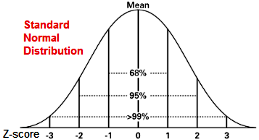
The values of any normal distribution can be translated into a standard normal distribution, meaning that any distribution can be re-scaled into a curve centered in the value of zero. This process is called standardization and given that the goal is to construct a Z-distribution, the resulting values corresponding to each point in the Z-distribution are named Z-scores. The formula to obtain such Z-scores is:
Where:
-score or standard score
original value from the original normal distribution
mean of the original distribution
standard deviation of original distribution
In other words, every single outcome resulting in a statistical experiment of a continuous random variable can be re-scaled into a standard score. This standardization allows the systematic estimation of the probability of events from any set of normal distributions, which in turn helps to compare within more than one of these normal distributions.
Usually when studying a large population, statisticians look for the greatest amount of information possible to be gathered from such population, the higher the volume and the amount of variables to study, the higher the knowledge of the population in question. But the problem with this is that most researchers will end with a set of varied data distributions, each with a different mean and standard deviation, making the comparison and calculation of probabilities of specific outcomes from multiple distributions to be not only complicated, but tedious. The solution is to use standardization to translate or re-scale all of the different distributions in order to work with such multiple data sets and recollect information as a whole.
This process allows researchers of large populations to obtain a more complete picture of the population, and making the process faster and efficient.
How is this done? We will go into detail on the mathematical calculations for re-scaling a normal distribution into a Z-distribution in the next section. For now, you just need to know that the whole ordeal requires you to rescale values of each original normal distribution being used into a standard score (or Z-score), use these values to construct the standard normal curve (Z-distribution curve) resulting for each of the original distributions, then you can calculate the probability of different events related to each different variable distribution. When having many data distributions all with the same scale, you can now compare the probability of events associated with each of them if you want, or need to. Important values associated with probabilities and z-scores can be found in the Z scores table (we have added two Z- tables) depicted below:
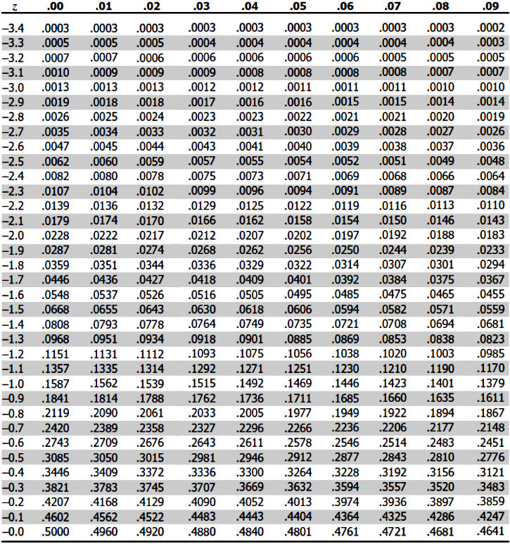
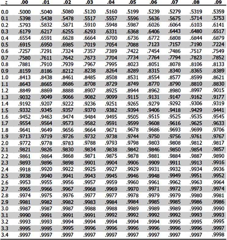
Usually, only one big Z-table is used (which contains all from figure 2 and 3), but for practical purposes we have divided it in the one for negative z scores and positive z scores.
How to find z scores?
Now lets take a look at how to work through the standardization process and using equation 1 to obtain Z scores. For that, we will solve a few example problems, the first an second problems focus on the process of translating a normal distribution into a standard normal distribution, while the third problem focuses on finding raw data from Z-scores. Have fun!
Example 1
The heights of a population of women are normally distributed. The mean height is 164 cm with a standard deviation of 8 cm. What is the probability of a randomly selected woman who is shorter than 169 cm in this population?For this question, we are looking for the area under the bell curve which contains values below the 169 cm mark in the original normal distribution, therefore, we need to find where this mark is in the standard normal distribution to then find the probability of such sub interval using the Z-table.
Using equation 1 to calculate the Z score related to the value of . We have that:
and
Then:
This means that the probability of randomly selecting a woman who is shorter than 169 cm in this population is equal to the area under the curve of the standard normal distribution as shown below:
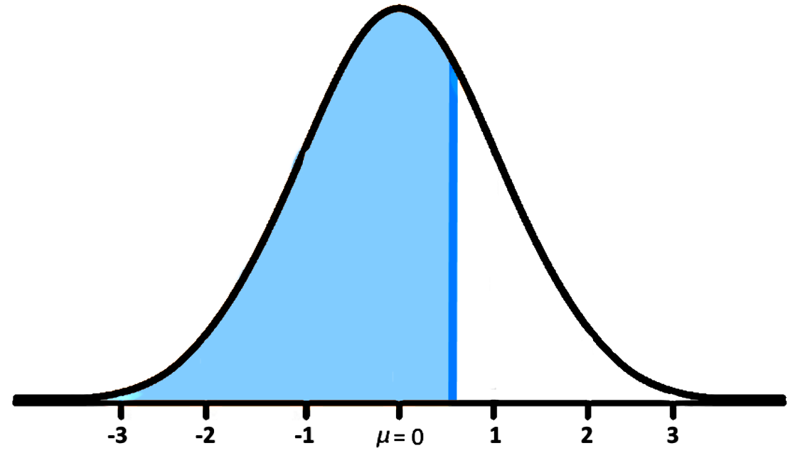
Now, to find the probability value we use the Z-tables provided above:
- For this case you will use the Z-table for a positive Z-value which is depicted in figure 3.
- Go to the row containing the first digit, and the first digit of the decimal point of your Z-value obtained in equation 2.
- Then go to the column containing the second digit after the decimal point of your Z-value from equation 2.
- Notice that since we have a third digit after the decimal point in our Z-value, the best probability we can obtain is a close approximation. So we know that our probability of choosing a woman shorter than 169 cm is not exactly the value where the row and column specified above intersect, the real value should be a little bit to the right but not quite the following value; therefore, the probability of this event is between 0.7324 and 0.7357.
Following the last steps, we know that a good approximation value for the probability of randomly selecting a woman who is shorter than 169cm is 0.734, or P(Z < 0.625) 0.734.
Example 2
The age at which a group of children first started talking is normally distributed. The data set has a mean of 18 months and a standard deviation of 2.3 months. What is the percentage of this group of children who first started talking between 15 and 24 months?Since we want to find the percentage of children within a specific subinterval within the whole distribution, we need to calculate the Z-scores of the two limits in order to identify the subinterval in the Z-distribution. Finding Z scores related to the values of and where we have that: and can be done using equation 1 as follows:
For :
For :
With these values, we now can see the percentage of children who learnt to talk within the 15 and 24 months of age depicted in the standard normal distribution below:
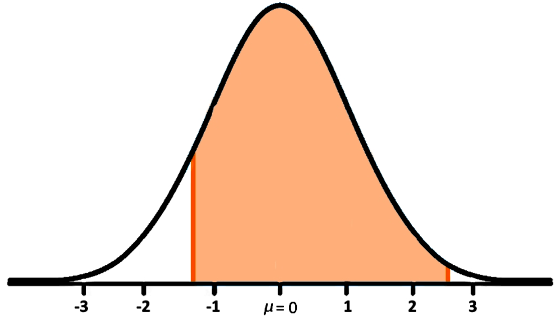
Now, to find the value that this percentage represents, we need to use the Z-tables provided in figures 2 and 3:
- To start, remember that if we were to divide the standard normal distribution using the mean (value of zero) each side of the graph will equate to a value of 50% which is a probability of 0.5 for the area under the curve. This is important to remember because we will be using this logic to find the area under the curve shown in figure 5.
- First let us find the percentage of children who learnt how to talk at 24 months of age. For that, we use the Z-table in figure 3 (with the positive Z-score values).
- We go to the row with the 2.6 Z value.
- Then we use the column corresponding to the 0.01 value.
- We intersect this row and column and find that the probability of children who talk by age 24 months is equal to 0.9955, which equates to 99.55% of children.
- Then we find the percentage of children who talk by age 15 months.
- Using the Z-table in figure 2, we go to the row with the -1.3 Z value.
- Then we use the column corresponding to the 0.00 value.
- We intersect this row and column and find that the probability of children who talk by age 15 months is equal to 0.0968, which equates to 9.68% of children
- Therefore, we can just subtract the percentage of kids who talk by age 15 from the percentage of kids who talk by age 24 to obtain: 99.55 - 9.68 = 89.87.
And so, the percentage of children to learn how to speak between 15 and 24 months of age from this group is approximately equal to 89.87%.
Example 3
An environmental group did a survey on how much water a population consumed when taking shower and bath. It was found that the amount of water consumption is normally distributed with a mean value of 65 liters and a standard deviation of 4.3 liters. What is the amount of water that separates the least 90% from the most 10%?On this case we want to know the mark in the original normal distribution curve that delimits the area under the distribution curve that covers 90% of the population (the 90% that uses the least water) and the 10% of the population that uses the most water. Or in other words, we want to know what is the amount of water (in liters) that 90% of the population uses at the most, when taking a shower and bath.
For that, you need to find the value on the distribution interval that will produce a probability of 90% area under a curve from a Z-distribution. For that, we go to figure 3 at the Z-table for positive values of Z and check which value of Z would provide a probability of 0.9. The closest match is shown below:
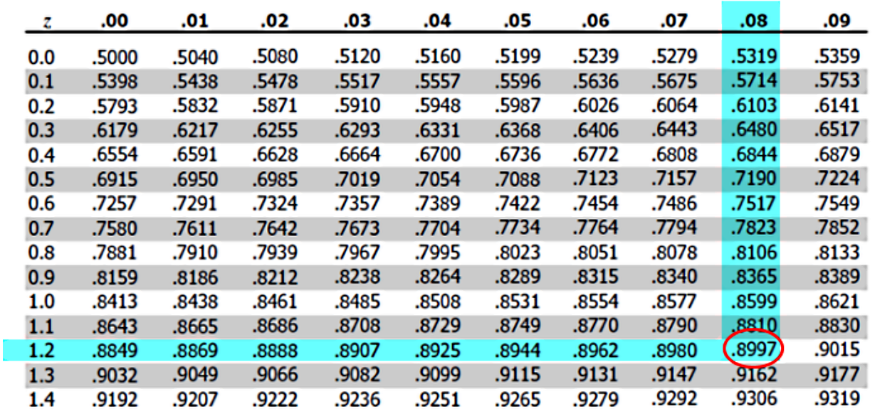
Therefore, the Z-score associated with 90% of the population is 1.28. Let us translate this into a regular normal distribution, to know the real value in liters that 90% of the population use at the most, for that, we use equation 1 and solve for x.
So, we have that: and , therefore:
Which means that the water consumption mark that separates the lower 90% of the population from the higher 10% of the population is the 70.504L mark. Or in other words, 90% of the population consume at the most 70.504L of water when taking a shower and bath.
To finish up with this lesson we recommend you to take a look at this handout on Z-scores which gives a fun way to learn about the importance of standard normal distributions and standard scores.
We hope you have enjoyed this lesson, see you on the next one!


