Introduction to normal distribution
Thanks to our past lessons on the probability distribution - histogram, mean, variance and standard deviation you are already familiarized with the concept of a probability distribution: A tool that allows us to understand the values that a random variable may produce by providing a graphic representation of all the possible values of such random variable and the probability of each of them occurring.
With this in mind, remember that random variables are classified into two categories depending on the type of values they can contain: Discrete random variables and continuous random variables.
A discrete random variable is that which contains countable values: whole numbers, integers. Therefore, discrete random variables refer to variables that deal with items that can be counted as complete units, not fractions or any infinitesimally small parts of a unit interval. On the other hand a continuous random variable can have any possible value, as long as it belongs to a particular defined interval that is being studied. Simply said, a continuous random variable can assume any value within a specified interval of values, that means that once you have set the starting and ending point, the continuous variable can have values with decimal expressions or fractions. Continuous random variables are said to be continuous because they will contain every single value within the interval, and that means that not matter how small you scale your interval, this variable is taking account of every single infinitesimally small point in it.
On this lesson we will make use of continuous random variables since they will be the ones producing a continuous probability distribution, also known as the normal distribution.
What is a normal distribution?
As mentioned above, a normal distribution is a continuous probability distribution, which happens to be the most widely used continuous probability distribution that there is!
Also called a Gaussian distribution, it allows an statistician to work with the best approximation for a random variables behavior from real life scenarios since it has been established in the central limit theorem that as long as the sample is sufficiently large, the shape of a random variables distribution will be nearly normal.
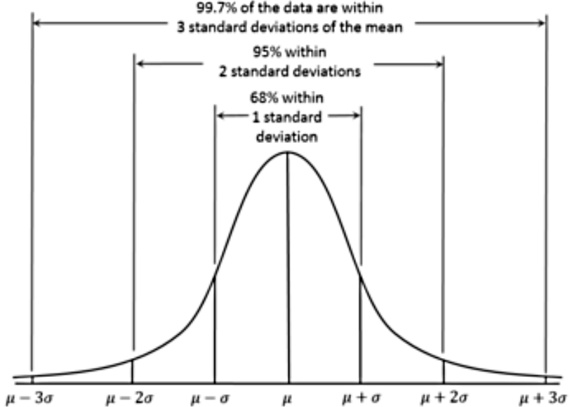
The normal distribution graph looks like:
Properties of a normal distribution
The main characteristics of a normal probability distribution are:
- It has a bell-shaped curve (reason why many times is simply called a bell curve, or a bell distribution).
- The bell curve is symmetric with the mean of the distribution as its symmetry axis and this mean has a value that is equal to the median and mode of the distribution (so, median = mode = mean in a normal distribution!).
- The bell represents the whole probability distribution of a continuous random variable, therefore, the area under the curve is equal to 1 because the event we study with such probability distribution will occur within the interval of the distribution. Since the total area under the curve is equal to 1, then half of it is on one side of the mean value (the axis of symmetry) and half is on the other side.
- The left and right tails of the normal distribution never touch the horizontal axis, they extend indefinitely because the distribution is asymptotic.
- The shape of the normal distribution and its position on the horizontal axis are determined by the standard deviation and the mean. The mean sets the center point, while the bigger the standard deviation, the wider the bell curve will be.
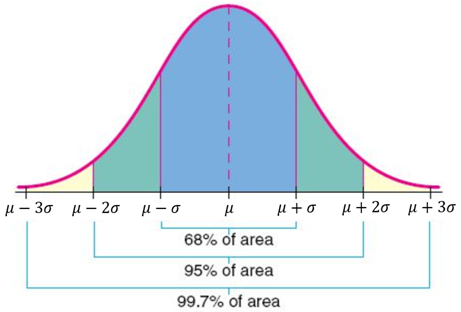
- About 68% of the population are within 1 standard deviation of the mean.
- About 95% of the population are within 2 standard deviations of the mean.
- About 99.7% of the population are within 3 standard deviations of the mean.
Normal distribution examples
For this lesson we will take a look at a single problem on normal distributions, but this will be enough to showcase multiple examples of the distribution curve and the portions of it we can identify thanks to knowing about its mathematical properties. Notice we have not introduced a normal distribution formula yet, we will leave most probability calculations to laters lessons, let us focus on the properties of the distribution today. So, let us start!
Example 1
The weight of chocolate bars produced by a factory is normally distributed with a mean of 225 grams and a standard deviation of 5 grams. Determine the percentage of the chocolate bars that could be expected to weigh- between 220 and 230 grams.
- between 215 and 235 grams.
- between 210 and 240 grams.
- between 225 and 230 grams.
- between 230 and 235 grams.
- between 210 and 215 grams.
- between 220 and 240 grams.
- above 225 grams.
- above 240 grams.
- below 220 grams.
For this problem let us construct a normal distribution curve where we have identified the value provided for the mean and the plus or minus standard deviations:
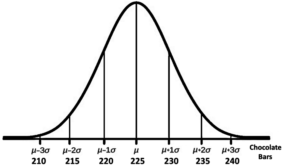
Remember that the normal distribution definition tells us the curve is symmetric by having the line delimited by the mean value as the axis of symmetry, therefore, the quantity found on the left hand side of the mean is exactly equal to the quantity on the right hand side of the mean. With that in mind, let us answer each of the ten parts of this problem, in each part we will show the graphic representation of the portion of the graph in question.
For parts a), b) and c):
We know that a chocolate bar weight between 220 and 230 grams happens to be the range of values within one standard deviation from the mean of the distribution, represented in the graph below in yellow.
In the same way, we know that a range of 215 to 235 grams of weight is the range contained within 2 standard deviations from the mean in the distribution (represented in the graph below in cyan), and the range of 210 to 240 grams is contained within 3 standard deviations from the mean in the distribution (represented in pink in the graph).

Thanks to the properties of the normal distribution we know that all normal distribution curves follow the rules of percentages of distribution throughout the extent of their standard deviations as shown in figure , and therefore to answer parts a), b) and c) we have that:
- 68% of chocolate bars are between 220 and 230 grams.
- 95% of chocolate bars are between 215 and 235 grams.
- 99.7% of chocolate bars are between 210 and 240 grams.
For part d)
We know that from 225 to 230 grams is half the range between one standard deviation within the mean:
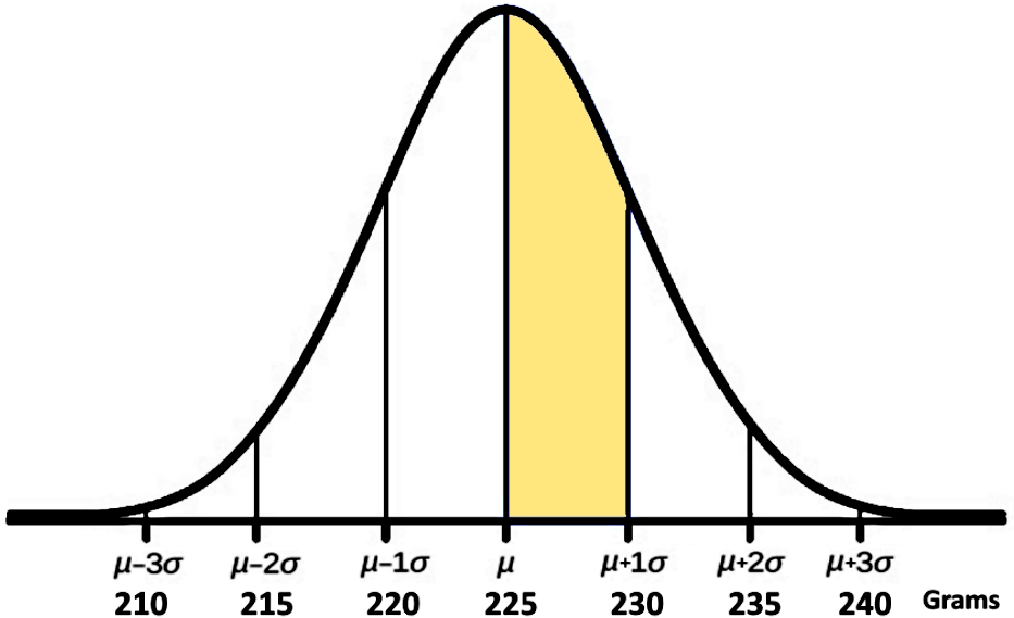
Since the range within one standard deviation from the mean comprised 68%, then half of it comprises 34%.
For part e)
Since the range between 230 and 235 grams of weight comprises the range within plus one standard deviation and plus two standard deviations in the distribution curve (as shown in the figure below), we have to use the total range comprised from minus to plus two standard deviations, which we know is 95% and subtract from it until we have the desired piece of the distribution.
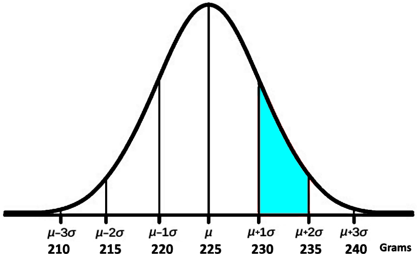
Now that we can see figure 5, we can easily notice that if we can take the 95% corresponding to the range of 215 to 235 grams, divide it in two to obtain 47.5% corresponding to the range from 225 to 235 grams. From that, we subtract the 225 - 230 range found in part d above, which is equal to 34%. Therefore we have that 47.5%- 34% = 13.5% .
And so, the percentage corresponding to the range between 230 and 235 is 13.5%.
For part f)
Looking for the percentage of chocolate bars that weight within 210 and 215 grams.
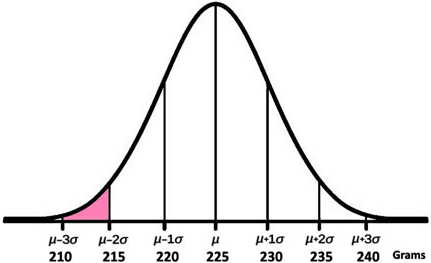
In this case there are three important things to notice:
We already know that 99.7% of the chocolate bars weight between 210 to 240 grams, we can divide it by two and obtain that a 49.85% of the chocolate bars weight within 210 to 225 grams.
Then, we know that the range comprising from 215 to 225 grams corresponds to the exact same percentage of chocolate bars than the ones weighting within the range of 225 and 235 grams, which we know from part e) that equals to 47.5%.
And so, we just subtract these two numbers: 49.85%-47.5%=2.35% , and we obtain that only 2.35% of the chocolate bars weight within 210 to 215 grams.
For part g)
The part of the distribution containing the chocolate bars that weight within 220 and 240 grams can be seen below:
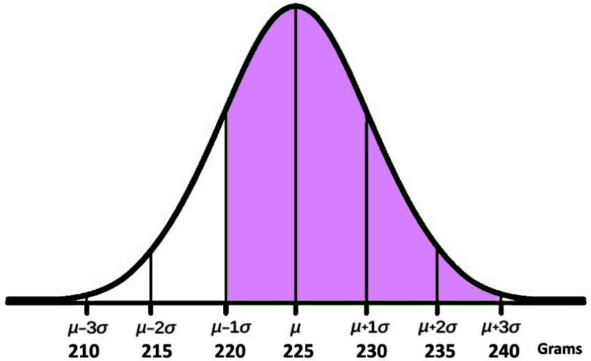
Since we know that 49.85% of the chocolate bars weight within 225 and 240 grams (obtained in part f), and we know that 34% of the bars weight between 220 and 225 grams (obtained in part d), we just add those two numbers: 49.85%+34%=83.85%.
For part h)
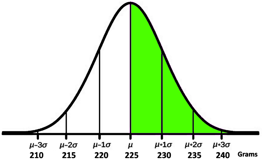
Since the mean weight of the chocolate bars for this normal distribution is 225 grams, notice that all of the chocolate bars that weight above above 225 grams represent half of the entire amount of bars produced by the factory. Thus, this is simple, 50% of the chocolate bars weight more than 225 grams and you can see this represented in the figure below:
For part i)
The portion of chocolate bars that weight above 240 grams is represented in the next figure:
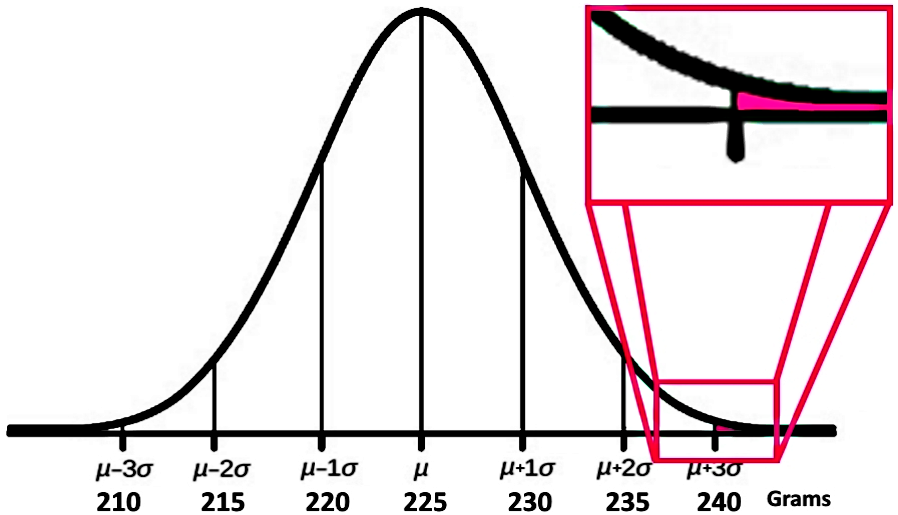
Notice that this proportion of chocolate bars is three standard deviations away from the mean weight, therefore, they represent a very small portion of the entire chocolate bar production.
If we know that in normal distributions about 99.7% of the population are within 3 standard deviations of the mean, that means that what is left out of the three standard deviations from the mean is equal to 100% - 99.7% = 0.3%.
Remember, this 0.3% that is left is distributed in both sides of the distribution (either before the value equal to the mean minus three standard deviations, or after the value equal to the mean plus three standard deviations); therefore, the portion of chocolate bars that weight above 240 grams is equal to the 0.15% of the entire production.
For part j)
The portion of the chocolate bars that weight below 220 grams can be seen in the figure below:
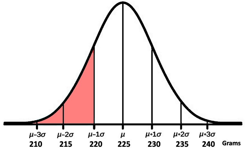
To obtain this piece of the distribution we just subtract 34% corresponding to the range between 220 to 225 grams to the 50% on the left hand side of the mean, producing a result of 16% for the range contained below the value of 220 grams.
As you can see, throughout this lesson we just wanted you to familiarize yourself with what a normal distribution function is, its graph shape, and the properties of it. Now that you know how to find answers by studying a bell-shaped distribution, it is time to learn more about the relationship between the area under this bell curve and probability. Thus, we will go to our next lesson on normal distribution and continuous random variables, where we will finally introduce a normal distribution equation and work on calculations for probability.
For now, this is the end of our lesson, we recommend you to take a look at this handout which also provides an introduction to the normal distribution and curve, since it contains a nicely presented summary of our topic for today and it may be useful to you while studying.
See you in our next lesson!
Properties of a Normal Distribution
About 68% of the population are within 1 standard deviation of the mean.
About 95% of the population are within 2 standard deviations of the mean.
About 99.7% of the population are within 3 standard deviations of the mean.
.
Calculator Commands
To calculate the normal distribution probability between two data values:
normalcdf (lower bound, upper bound, mean, standard deviation)
- To calculate the area to the left of a data value, replace the lower bound by
- To calculate the area to the right of a data value, replace the upper bound by
To calculate a data value, given the area to the left of the data value:
invNorm (area, mean, standard deviation)
About 68% of the population are within 1 standard deviation of the mean.
About 95% of the population are within 2 standard deviations of the mean.
About 99.7% of the population are within 3 standard deviations of the mean.
.

Calculator Commands
To calculate the normal distribution probability between two data values:
normalcdf (lower bound, upper bound, mean, standard deviation)
- To calculate the area to the left of a data value, replace the lower bound by
- To calculate the area to the right of a data value, replace the upper bound by
To calculate a data value, given the area to the left of the data value:
invNorm (area, mean, standard deviation)


