Geometric Distribution: Probability Formulas and Real-World Applications

Dive into geometric distribution concepts, formulas, and practical examples. Understand its relationship with binomial distribution and master probability calculations for various scenarios.

Geometric distribution

To continue with the detailed study of discrete probability distributions we will focus our lesson of today on the geometric probability distribution. You will notice that this type of discrete distribution shares many of its characteristics with the binomial distribution, so make sure to pay attention to the different details of them so you can distinguish and solve accordingly when working on assignments and in your independent studies.

Geometric probability distribution

A geometric distribution is that which describes the probability distribution of the number of trials in an experiment needed for the expected event (that which we are looking for, or that which we call success) to occur. In simple words, we define geometric distribution as that which expresses the probability of an expected outcome to occur within a range of a particular amount of trials, and once it does, the experiment stops (he experiment is only looking for the first success, afterwards, no more trials are needed).

Since we will be performing a number of trials before an outcome defined as success occurs, there is no limit on how many trials can occur before the success arrives. The number of trials run up to a first success (all the ones resulting in failures, plus the one resulting in the first success) is what we call the geometric random variable $n$ (see equation 1).

It is important to mention that each individual trial has the same probability of producing a success. This means that every trial is run with all of the possible outcomes inside, or what is usually called with replacement; meaning that no matter how many trials are performed, every single time one is done, if its result was a failure, this value is thrown back (or remains) in the pool of possible outcomes for the next trial to work with it again.
The easiest example of this is an experiment with a fair die: since every time you roll a die you have a $\frac{1}{6}$ of probability of obtaining any of the 6 numbers of its faces; no matter how many times you roll the die, if the first attempt resulted in a 2, the value of 2 is possible once again in the next roll with exactly the same probability on that particular trial as in the one before because there is no way to take away the value of 2 from the possible outcomes pool without destroying or modifying the die.

Another thing worth nothing is that the geometric distribution has a memoryless property, which means that you can do the experiment until you obtain a success, and then re-do the entire experiment once again without taking into account the failures that occurred on the first experiment (they do not affect the second experiment or its geometric function at all) and the system is taken as if it has no memory of the first experiment ever happening. How? Well since every experiment is defined as running trials until a success occurs, once you redo the experiment again there hasnt been any successes yet, therefore, the scenario for the observation of the probability distributions behaviour is reseted and is as if the failures and the one success from the first experiment had never happened. This may sound as something we could take as a given, but in reality only two probability distributions share this characteristic, and the other one is a continuous distribution: the exponential distribution.

And so, we focus on finding how many trials are needed to obtain a success, for that, the probability distribution formula for a geometric distribution, or the mathematical expression for the probability of getting a first success in the nth trial, is defined as:

$P(n) = (1-p)^{n-1}p$
Where:
$n$ = number of trials until the first success
$p$ = probability of success in each trial
$P(n)$ = probability of getting your first success in the $n^{th}$ trial

Just as in a binomial distribution, in a statistical experiment defined by a geometric probability distribution there are only two possible outcomes: failures or successes, and the probability of success must be the same throughout every single trial (independence is necessary).
You will see similar sharing of characteristics within the other discrete probability distributions in our past lessons, but as always, these discrete distributions have been classified as different given the approach they use to solve for the probabilities of an expected event (or success).

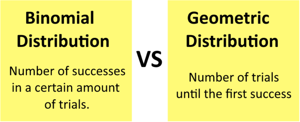
Between the binomial and the geometric distribution, the difference lies in that the binomial distribution looks for the probability of obtaining an $x$ amount of successes out of an n amount of trials, while the geometric distribution focuses on the amount of trials needed to obtain a success.


The fact that a binomial distribution can count more than one success in a certain amount of trials without restarting the experiment makes it impossible for it to have the memoryless property, like the geometric distribution.

Geometric distribution examples

Now let us work on a few examples to understand in a deeper way what the geometric distribution is:

Example 1

Identify which of the following experiments below are geometric distributions:

This is a geometric distribution where the success outcome is heads. This can be easily seen when they say the experiment will be performed until the success occurs, and then it studies the probability of this taking 5 trials.

This is not a geometric distribution since is talking about a number of successes in a particular amount of trials, note how the experiment is not meant to be stopped once the success happens, there will be 5 trials run no matter when and if the success occurs. This looks more like a binomial distribution.

This distribution cannot be a geometric distribution because the trials are run without replacement, which changes the probability of a success in each individual trial.

This is a geometric probability distribution because is looking for the probability of finding the first success on a certain trial, and once the successful trial is done, the experiment restarts without memory.

Example 2

Let us use the last case from example problem 1 and solve for the probabilities:
There is a certain machine that produces knick-knacks. This machine produces a defective knick-knack with probability 0.1. What is the probability that this machine will produce its first defective knick-knack on the 8th knick knack it produces?

On this case $p=0.1=\frac{1}{10}$ and $n=8$. Using the geometric distribution formula shown in equation 1 for the probability of a first success at an nth trial, we calculate:

$P(n) = (1-p)^{n-1} p \,$→$\, P(n=8) = (1-\frac{1}{10})^{8-1} (\frac{1}{10})$
$P(8) = (1-\frac{1}{10})^{8-1} (\frac{1}{10}) = (\frac{9}{10})^{7}(\frac{1}{10}) = (\frac{9}{10}) (\frac{9}{10})(\frac{9}{10})(\frac{9}{10})(\frac{9}{10})(\frac{9}{10})(\frac{9}{10})(\frac{1}{10}) = (\frac{4782969}{100000000}) = 0.0478$
Therefore, there is a 4.78% chance that the machine will produce a defective knick-knack on the 8th knick-knack produced.

Example 3

In the game Dungeons and Dragons a fair 20 sided die (icosahedron, plural: icosahedra) is used. A critical hit is when a 20 is rolled.

Since the icosahedron is fair and we are talking about the first attempt, the probability of throwing a critical hit should be the same as the probability of throwing a hit at any single attempt: $p=\frac{1}{20}$. To prove this, let us calculate it using equation 1:

$P(n) = (1-p)^{n-1} p \;$→$\; P(n=1) = (1-\frac{1}{20})^{1-1} (\frac{1}{20})$
$P(1) = (1-\frac{1}{20})^{1-1} (\frac{1}{20}) = (\frac{19}{20})^{0}(\frac{1}{20}) = 1(\frac{1}{20}) = \frac{1}{20} = 0.05$
Since the question is asking for the probability of success in less than three rolls of the icosahedron, we need to find the probability for a critical hit to happen in the first two rolls; for that, we add the probability of success in trial one and the probability of success in trial two:

$P(n < 3 ) = P(n=1) + P(n=2) = P(1) + P(2)$
Since we already have $P(1)$ from part 1, we calculate $P(2)$:
$P(n) = (1-p)^{n-1} p \;$→$\; P(n=2) = (1-\frac{1}{20})^{2-1} (\frac{1}{20})$
$P(2) = (1-\frac{1}{20})^{2-1} (\frac{1}{20}) = (\frac{19}{20})^{1}(\frac{1}{20}) = (\frac{19}{20}) (\frac{1}{20}) = \frac{19}{400} = 0.0475$
therefore:
$P(n < 3 ) = P(1) + P(2) = 0.05 + 0.0475 = 0.0975$

Example 4

Balls are drawn with replacement from an urn containing 9 black balls, and 1 golden ball.

Since there are 10 balls in total and all of them have the same probability of being drawn on any trial, the probability of success in each trial is $p=\frac{1}{10}$. Since the question asks us about the probability of success in the first trial, our value of $n$ is $n=1$. Therefore, to calculate the probability we compute:

$P(n) = (1-p)^{n-1} p \;$→$\; P(n=1) = (1-\frac{1}{10})^{1-1} (\frac{1}{10})$
$P(1) = (1-\frac{1}{10})^{1-1} (\frac{1}{10}) = (\frac{9}{10})^{0}(\frac{1}{10}) = 1(\frac{1}{10}) = \frac{1}{10} = 0.1$
And so, we can observe once more that since this question is focused on the first trial, the probability is equal to the simple probability of success in each trial $P(1)=\frac{1}{10}=p$.

Using equation 1 with $n=2$ for this case, and following the same process as in part 1, we calculate:

$P(n) = (1-p)^{n-1} p \;$→$\; P(n=2) = (1-\frac{1}{10})^{2-1} (\frac{1}{10})$
$P(2) = (1-\frac{1}{10})^{2-1} (\frac{1}{10}) = (\frac{9}{10})^{1}(\frac{1}{10}) = (\frac{9}{10}) (\frac{1}{10}) = \frac{9}{100} = 0.09$
Notice how the probability reduces as trials go by because of the nature of the experiment where balls are drawn with replacement.

Repeating the process done before, now with $n=3$.

$P(n) = (1-p)^{n-1} p \;$→$\; P(n=3) = (1-\frac{1}{10})^{3-1} (\frac{1}{10})$
$P(3) = (1-\frac{1}{10})^{3-1} (\frac{1}{10}) = (\frac{9}{10})^{2}(\frac{1}{10}) = (\frac{9}{10})(\frac{9}{10})(\frac{1}{10}) = \frac{81}{1000} = 0.081$

And to finalize with this problem, we calculate the probability of obtaining the golden ball on one of the first 5 draws. For that, we add up the probabilities of finding the golden ball first at trial 1, trial 2, trial 3, trial 4 and trial 5.

$P(n \leq 5 ) = P(1) + P(2) + P(3) + P(4) + P(5)$
So far we already have the first three numbers, since we got them in part 1 through 3 of this problem, therefore, let us calculate $P(4)$ and $P(5)$:

$P(n) = (1-p)^{n-1} p \;$→$\; P(n=4) = (1-\frac{1}{10})^{4-1} (\frac{1}{10})$
$P(4) = (1-\frac{1}{10})^{4-1} (\frac{1}{10}) = (\frac{9}{10})^{3}(\frac{1}{10}) = (\frac{9}{10})(\frac{9}{10})(\frac{9}{10})(\frac{1}{10}) = \frac{729}{10000} = 0.00729$
and
$P(n) = (1-p)^{n-1} p \;$→$\; P(n=5) = (1-\frac{1}{10})^{5-1} (\frac{1}{10})$
$P(5) = (1-\frac{1}{10})^{5-1} (\frac{1}{10}) = (\frac{9}{10})^{4}(\frac{1}{10}) = (\frac{9}{10})(\frac{9}{10})(\frac{9}{10})(\frac{9}{10})(\frac{1}{10}) = \frac{6561}{100000} = 0.06561$
Therefore, the total probability of finding the golden ball in any of the first five attempts is:

$P(n \leq 5 ) = P(1) + P(2) + P(3) + P(4) + P(5)$
$P(n \leq 5 ) = 0.1 + 0.09 + 0.081 + 0.0729 + 0.06561$
$P(n \leq 5 ) = 0.40951$
Check the videos on this lesson where you can see the process of calculating these probabilities using the calculator.

*** To finalize the lesson of today, we recommend you to visit the next lesson on geometric and binomial distributions , which can help you to reaffirm what you have learned so far on these last two lessons. For another perspective on the geometric distribution, these statistics lectures provide a nice example and computation to analyze in detail.

This has been all for the lesson of today, we hope you enjoyed it and will see you in the next one!