Chi-Squared Critical Values: Mastering Statistical Analysis

Unlock the power of chi-squared critical values in statistical analysis. Learn calculation methods, interpret results, and apply them to real-world scenarios. Boost your confidence in hypothesis testing and data interpretation.

Chi - Squared confidence intervals

In todays lesson we will learn what is chi square in statistics and how do we use it when constructing confidence intervals.

What is chi square and what is a chi squared distribution?

A chi squared distribution comes from the chi square statistic, which measures how different are observed values from the expected ones from a true hypothesis in a statistical test. The chi square symbol is $x^{2}$, and this statistic is also called the goodness-of-fit statistic.

When talking in terms of the standard normal distribution, if we take a random sample of the values from such a distribution we would obtain a standard normal deviate. Squaring standard normal deviates and adding them together we would obtain a chi squared distribution, where the degrees of freedom are equal to the number of standard normal deviates that were added.

A Chi-Square with one degree of freedom is written as $x^{2}$(1), is simply the distribution of a single normal deviate squared. The area of a Chi Square distribution below 4 is the same as the area of a standard normal distribution below 2, since 4 is 2². The mean of a Chi Square distribution is its degrees of freedom. Chi Square distributions are positively skewed, as the degrees of freedom increase, the Chi Square distribution approaches a normal distribution.

The concept of the chi squared statistic can be a bit complicated so let us answer the following questions to have a little bit more insight on the matter:

• What is chi square distribution in statistics

Chi square goodness of fit test statistic is a measure of the difference between the observed values and the expected values squared from a sample obtained from a standard normal distribution.

• Does chi square assume normal distribution

No, is chi square distribution symmetric then? No, the curve for the chi square graph is skewed towards the right. A chi-square curve has no area associated with negative values and is asymmetric, with a longer tail on the right. There are actually many chi-square distributions, each one identified with a different number of degrees of freedom. Curves corresponding to several chi-square distributions are shown in Figure 1:


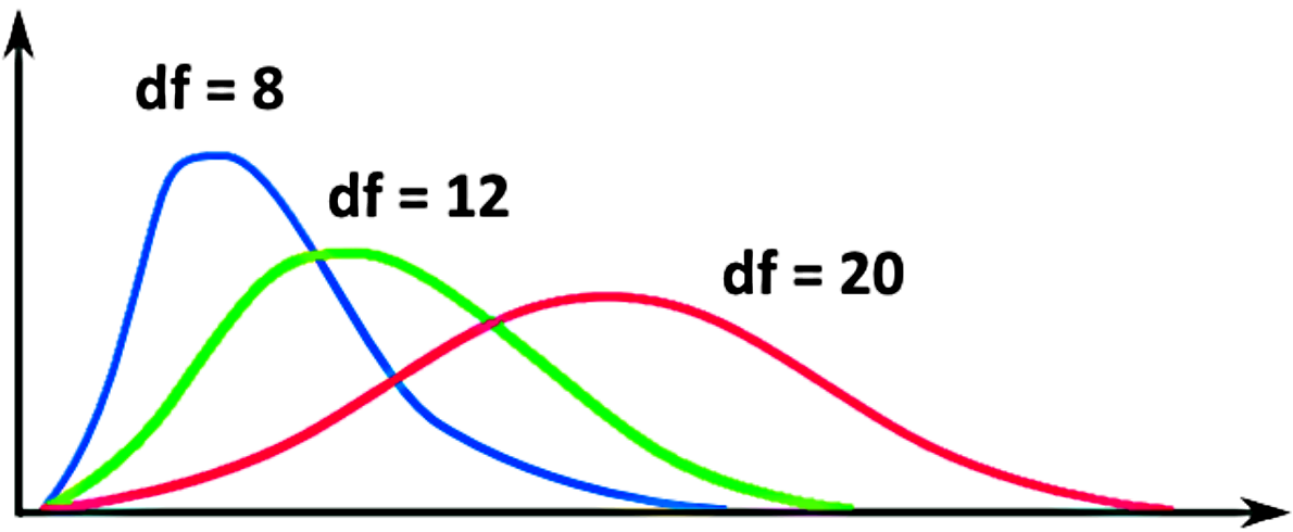
Notice the shape as the degrees of freedom increase, the more degrees of freedom present the more the chi-square curve looks almost symmetric like a normal distribution!

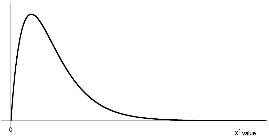
• What is the shape of the chi-square distribution?

A chi square distribution graph looks similar to a normal distribution but is skewed towards the right and it has all positive numbers in its horizontal axis. A general shape for a chi square is shown below:

• What is chi square critical value?

Just as for the normal distribution, when using a chi square distribution it is important to recognize some of its characteristics.

For example, when looking at what the area under the graph means we will find a confidence levell delimited by a confidence interval, and then a resulting significance level left on the side. Here is where the critical values come to place.

In any distribution, we know that a critical value is a point in the horizontal axis of the graph which marks the limit between an area (or region) and another. Usually, delimiting in between the confidence level ($n - \alpha$) and the significance level ($\alpha$). The chi square distribution follows the same rules and since the units of its horizontal axis is $x^{2}$ itself, we call these critical values: chi-square critical values.

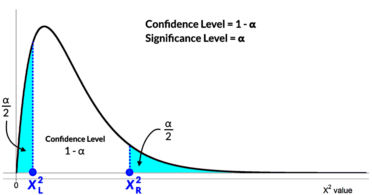
Notice in the graph below how the confidence level, the significance level and the critical values $X_{R} ^{2}$ and $X_{L} ^{2}$ are shown. The R and L subindexes denote the sides right and leftsince we are looking at a two tailed distribution, and notice the significance level is still evenly divided in halves (one for each side) even if the distribution is not symmetrical.


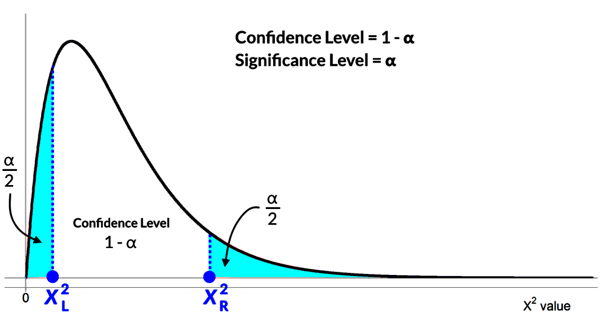
To find an area to the right of any critical value in the horizontal axis of this distribution such as $X_{R} ^{2}$ and $X_{L} ^{2}$ shown above, we use a chi-square distribution table. This table contains 3 types of values: degrees of freedom, area to the right of a critical value, and the chi square critical value itself and it looks like this:

Chi-square Table

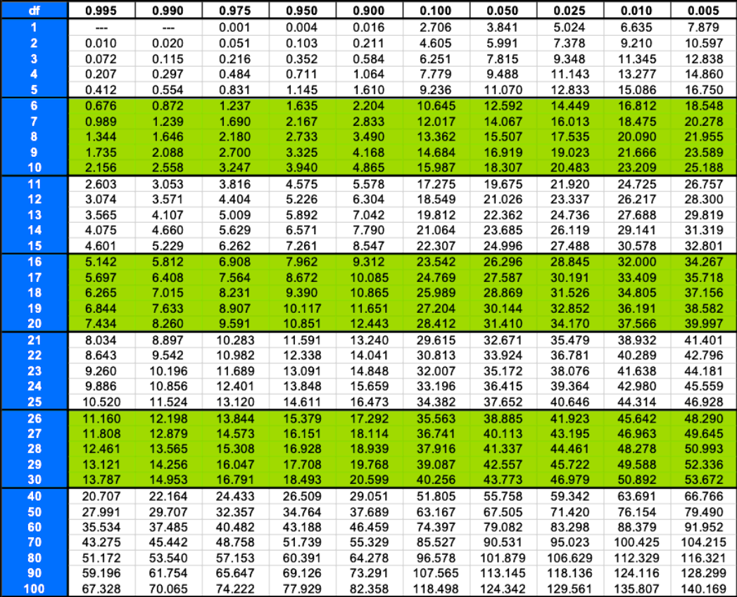
At the very left column of this chi squared table are the degrees, the top row contains the area values and the numbers inside this left-column/top-row frame are the chi square critical values. We will learn how this is used in a later section of the lesson.

An even bigger table (and more complete) can be found in the following link, and we recommend using it in conjunction with a chi square calculator (found at the end of this lesson) when solving multiple problems during studying time on your own.

When is chi square distribution used?

To estimate a population variance a Chi-Squared distribution is used,

Chi-Squared:

$\large X^{2} = \frac{(n-1)s^{2}}{\sigma^{2}}$
Where:
$X^{2}$ = chi square
$n$ = sample size
$s$ = sample standard deviation
$\sigma$ = population standard deviation
$\sigma^{2}$ = population variance
$n-1$ = degrees of freedom

From the chi square formula we can solve for the value of the variance (the square of the populations standard deviation).

With this we can calculate the confidence interval for that variance too, similarly to how we have used the t-distribution and the margin of error before to calculate the confidence interval for a population mean. The confidence interval, in this case for the variance or standard deviation squared, is given by:

$\large \frac{(n-1)s^{2}}{X_{R} ^{2}} < \; \sigma^{2} \; < \frac{(n-1)s^{2}}{X_{L} ^{2}}$
In this last formula, the chi square values in the denominators of each side refers to the chi square critical values defining the edges between the confidence level and the significance level on the distribution graph, and denoting that we have a two tailed significance level because we have a right side ($X_{R} ^{2}$) and a left side ($X_{L} ^{2}$) as shown below:


Another use for the chi-square distribution in statistics is when we are doing hypothesis testing, in this case, with the chi square test. We will talk about the chi-square test in a lesson later on.

How to use the chi square distribution table

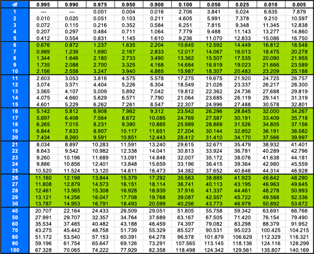
The Chi-Square table gives critical value area to the right:

Chi-square Table

Let me explain the chi square distribution table in a little more detail:
The first column to the left expresses the degrees of freedom for a particular situation, while the top row expresses the area to the right of any specific chi square critical value we are looking at.

Therefore, to find a value of chi square we look at the point in the table where the specific degrees of freedom row intersects with the column for the specific chi squared critical value. This process can be seen easily in example problem 2 on both parts a and b, so if you have any questions about how the chi square critical value table works, we recommend you to skip into that part of the lesson where you will also be reading about how to calculate chi square related confidence intervals.

How to solve chi square distribution

In order to understand better what chi square is and how we use it, let us take a look into a few problem examples.

Example 1:

Determining Degrees of Freedom
How many degrees of freedom does a sample of size,


The sample size is defined as $n=7$, and the degrees of freedom arise from simply subtracting $n-1$, therefore for this case the degrees of freedom are $n-1=7-1=6$.

And so we have 6 degrees of freedom in this case.


In this case $n = 20$.
Thus $n-1=20-1=19$.
19 degrees of freedom in this case.

Example 2:

Determining the Critical Value for a Chi-SquareDistribution ($X_{R} ^{2}$ and $X_{L} ^{2}$)
If a Chi-Squared distribution has 8 degrees of freedom find $X_{R} ^{2}$ and $X_{L} ^{2}$, with a


If we have 8 degrees of freedom, then this means that $n-1=8$, thus the sample size n is equal to 9.
A confidence level of 95% percent means $1 - \alpha = 0.95$, therefore the significance level is $\alpha = 1 - 0.95 = 0.05$.
This significance level is spread in two equal parts in two tails since we are asked for both $X_{R} ^{2}$ and $X_{L} ^{2}$, with this in mind, let us express that information in a chi squared distribution graph as follows:


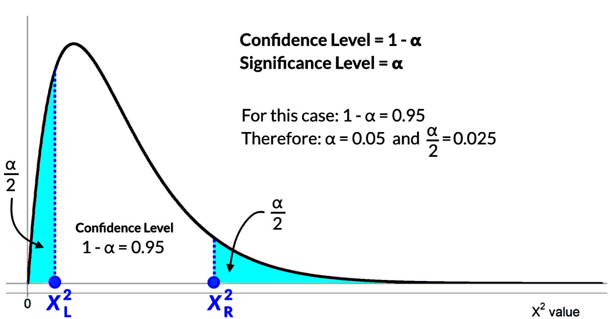
Using the information about the 8 degrees of freedom and the area value of half significance level we use the chi squared table to find the value of both critical values $X_{R} ^{2}$ and $X_{L} ^{2}$ .
Remember that the area value in the chi square table top row is the area to the right of a critical value, and so, we start with $X_{R} ^{2}$ since the area to its right is simply $\large \frac{\alpha}{2}$:

Therefore the right critical value is $X_{R} ^{2}$ =17.535.
Now, the area to the right of the left critical value is equal to the confidence level plus half alfa since it includes both the confidence level area and the right tail.
Area to the right of the left critical value:

1 $- \alpha +$ $\large \frac{\alpha}{2}$ = 0.95 + 0.025 = 0.975
We use this to obtain $X_{L} ^{2}$ :

Therefore the right critical value is $X_{L} ^{2}$ = 2.180 .


Remember we have 8 degrees of freedom, and in this case, a confidence level of 99% percent which means $1 - \alpha = 0.99$, therefore the significance level is $\alpha = 1 - 0.99 = 0.01$.

This significance level is spread in two equal parts in two tails: $X_{R} ^{2}$ and $X_{L} ^{2}$, and so we express that information in a chi squared distribution graph as follows:


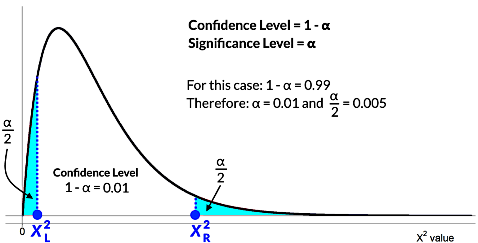
Using the information about the 8 degrees of freedom and the area value of half significance level we use the chi squared table to find the value of both critical values $X_{R} ^{2}$ and $X_{L} ^{2}$.
We start with $X_{R} ^{2}$ since the area to its right is simply $\large \frac{\alpha}{2}$:


Therefore the right critical value is $X_{R} ^{2}$ = 21.955 .
Now, the area to the right of the left critical value is equal to the confidence level plus half alfa since it includes both the confidence level area and the right tail.
Area to the right of the left critical value:

$1 - \alpha +$ $\large \frac{\alpha}{2}$ $= 0.99+0.005=0.995$
We use this to obtain $X_{L} ^{2}$:


Therefore the right critical value is $X_{L} ^{2}$ = 1.344 .

Example 3:

Determining the Confidence Interval for Variance
Road and racing bicycles have an average wheel diameter of 622mm. From a sample of 15 bicycles it was found that the wheel diameters have a variance of 10mm. With a 90% confidence level give a range where the variance of all road and racing bicycle wheels lie.

Let us gather all of the information of the problem:

$\quad n$= sample size = 15 bicycles
$\quad s$ = sample standard deviation thus $s^{2}$ = sample variance = 10 mm
$\quad \sigma$ = population standard deviation thus $\sigma^{2}$ = population variance
$\quad (n1)$ = degrees of freedom = 15 - 1 = 14 degrees of freedom.

Remember that the confidence interval of the variance is given by:

$\large \frac{(n-1)s^{2}}{X_{R} ^{2}} < \; \sigma^{2} \; \frac{(n-1)s^{2}}{X_{L} ^{2}}$
And so we need to find the critical values $X_{R} ^{2}$ and $X_{L} ^{2}$.
For that we use the 14 degrees of freedom and the confidence level of 90% given.
Since the confidence level is equal to 1 - $\alpha$= 0.90, we know that the significance level is $\alpha$ = 0.1 then, and $\large \frac{\alpha}{2}$ = 0.05.

We start with $X_{R} ^{2}$ since the area to its right is simply $\large \frac{\alpha}{2}$:


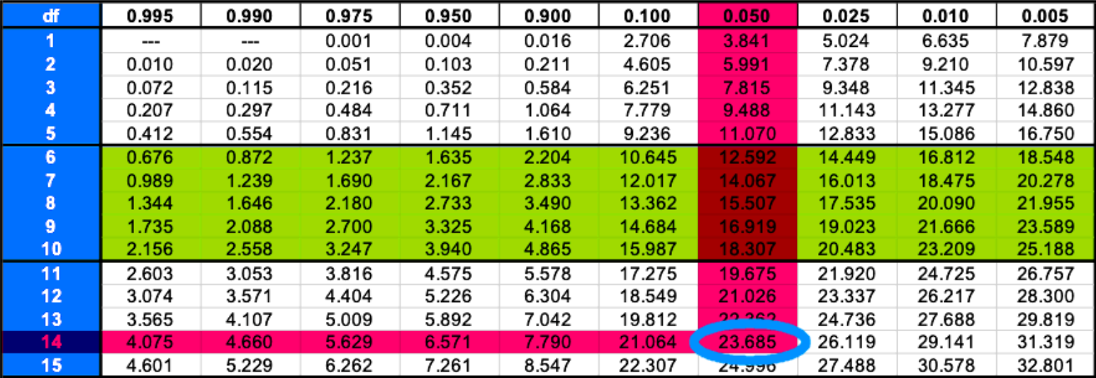
Therefore the right critical value is $X_{R} ^{2}$ = 23.685 .
Now, the area to the right of the left critical value is equal to the confidence level plus half alfa since it includes both the confidence level area and the right tail.
Area to the right of the left critical value:

1 -$\alpha$ + $\large \frac{\alpha}{2}$ = 0.90 + 0.05 = 0.95
We use this to obtain $X_{L} ^{2}$:


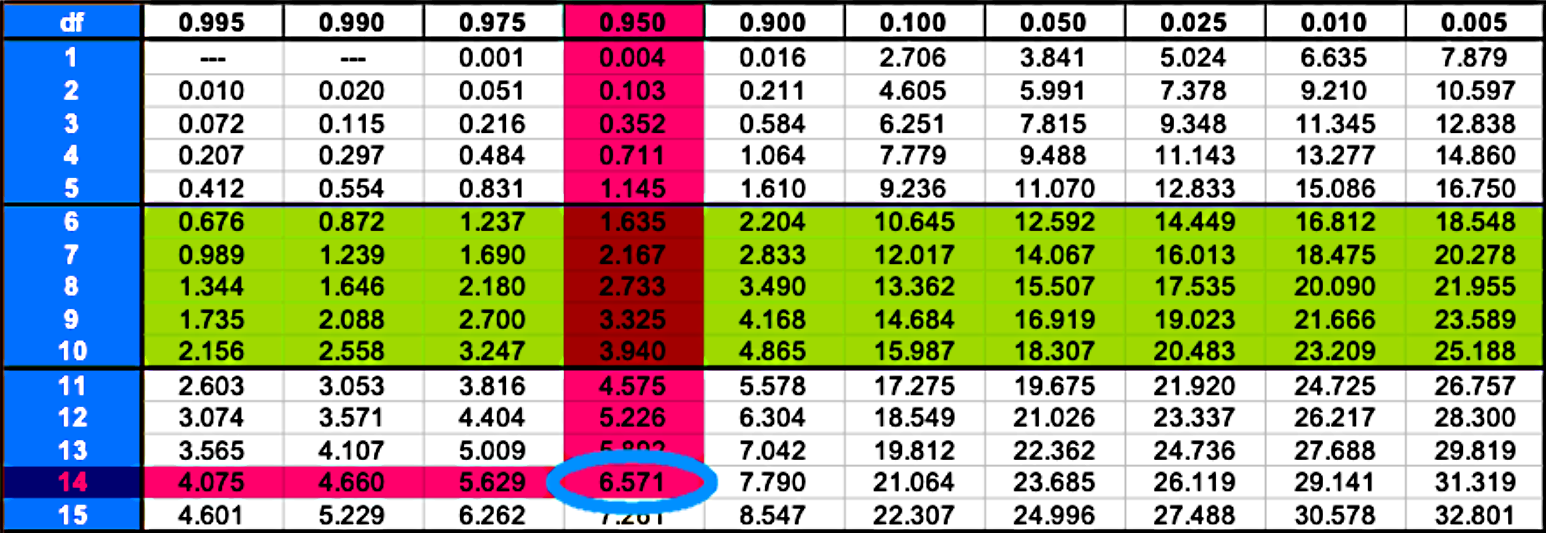
Therefore the right critical value is $X_{L} ^{2}$ = 6.571 .
And so finally we have everything we need to calculate the confidence interval for the variance:

$\large \frac{(n-1)s^{2}}{X_{R} ^{2}} < \; \sigma^{2} \; < \frac{(n-1)s^{2}}{X_{L} ^{2}}$
Where: $\large \frac{(n-1)s^{2}}{X_{R} ^{2}} = \frac{(14)(10)}{23.685} \approx$ $5.911$
And: $\large \frac{(n-1)s^{2}}{X_{L} ^{2}} = \frac{(14)(10)}{6.571} \approx$ $21.306$
Therefore:
$5.911 < \; \sigma^{2} \; < 21.306$

Example 4:

Determining the Confidence Interval for Standard Deviation
A Soda-pop company "Jim's Old Fashion Soda" is designing their bottling machine. After making 41 bottles they find that their bottles have an average of 335mL of liquid with a standard deviation of 3mL. With a 99% confidence level what is the range of standard deviation that this machine will output per bottle?

Let us gather all of the information of the problem:
$\quad n$= sample size = 41 bottles
$\quad \overline{x}$ = sample mean = 335 mL
$\quad s$ = sample standard deviation = 3 mL
$\quad s^{2}$ = sample variance = 9 mL²
$\quad \sigma$ = population standard deviation = thus $\sigma^{2}$= population variance
$\quad (n-1)$ = degrees of freedom = 41 - 1 = 40 degrees of freedom.

With all of this we are asked to find the confidence interval of the standard deviation of the population, but we only have the formula for the confidence interval of the variance which is given by:

$\large \frac{(n-1)s^{2}}{X_{R} ^{2}} < \; \sigma^{2} \; < \frac{(n-1)s^{2}}{X_{L} ^{2}}$
In order to obtain the formula needed, we use the fact that the population standard deviation is the square root of the variance, and so we have that:

$\large \sqrt{\frac{(n-1)s^{2}}{X_{R}^{2}}} \,< \, \sqrt{\sigma^{2}} \,< \, \sqrt{\frac{(n-1)s^{2}}{X_{L}^{2}}} \;$→$\; \frac{\sqrt{(n-1) \; \cdot \; s }}{X_{R}} \; < \; \sigma \; < \frac{\sqrt{(n-1) \; \cdot \; s }}{X_{L}}$
Where we have the degrees of freedom and the sample standard deviation, so we only need to find the critical values $X_{R} ^{2}$ and $X_{L} ^{2}$.

In this case we have 40 degrees of freedom and a confidence level of 99%, which is 1 - $\alpha$ = 0.99 and so the significance level is $\alpha$ = 0.01 and $\large \frac{\alpha}{2}$ = 0.005
We start with $X_{R} ^{2}$ since the area to its right is simply $\large \frac{\alpha}{2}$ :


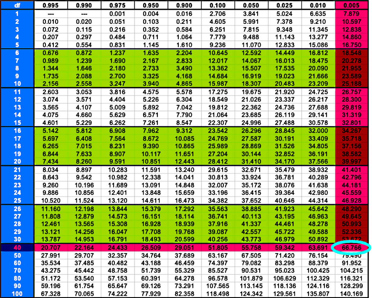
Therefore the right critical value is $X_{R} ^{2}$ = 66.766 .
For the left critical value we add the area for the confidence level plus half the significance level in the following manner:

1 - $\alpha$+ $\large \frac{\alpha}{2}$ = 0.99 + 0.005 = 0.995
We use this to obtain $X_{L} ^{2}$:


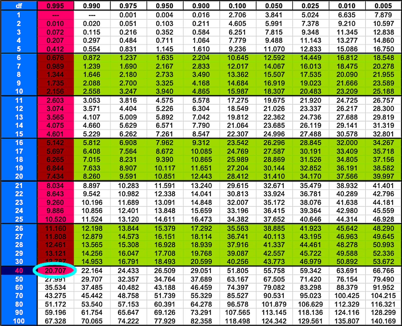
Therefore the right critical value is $X_{L} ^{2}$ = 20.707.
And so finally we have everything we need to calculate the confidence interval for the standard deviation:

$\large \frac{(n-1) \; \cdot \; s}{X_{R}} < \; \sigma \; < \frac{(n-1) \; \cdot \; s }{X_{L} }$
Where: $\large \frac{(n-1) \; \cdot \; s}{X_{R}} = \frac{\sqrt{40(3)}}{\sqrt{60.766}} \approx$ $2.322$
Where: $\large \frac{(n-1) \; \cdot \; s}{X_{L}} = \frac{\sqrt{40(3)}}{\sqrt{20.707}} \approx$ $4.169$
Therefore:
$2.322 < \; \sigma \; < 4.169$
And so, here ends our lesson but this is not the last time we talk about chi square. The question that comes to mind next is: Is chi square a test statistic? The answer lies in our hypothesis testing section of this course, where you will learn how you can perform a chi squared test.

Before you go, we would like to recommend the following chi square critical value calculator, so you can have a fast way to check your answers when using the methodology we have shown in this lesson.