


Diagonalization
Linear algebra diagonalization
Diagonalization is the process of taking a matrix and breaking it into a product of three distinct matrices. Although it sounds counterintuitive, breaking a matrix into a product of three matrices happens to be very useful when trying to find the high powers of a matrix.
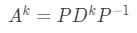
And so, if a matrix is diagonalizable, then it can be mathematically written as:
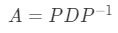
Where D is a diagonal matrix, and the convenience of this formula comes from the fact that it can help us find (when k is very big). This is due the relationship:

Given the components of equation 1 and 2, an important reminder is the computation of an inverse matrix which can be shown below:
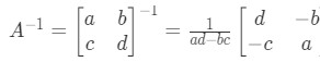
When finding the diagonalization of a matrix, you will use these three basic formulas plus a few other mathematical tools which will be mentioned in the next sections.
What is a diagonal matrix
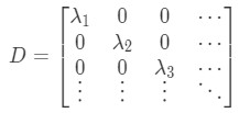
For this particular lesson is of utmost important that you are comfortable working with diagonal matrices. A diagonal matrix is that in which the entries on the main diagonal have values different than zero, and the rest of the values in the whole matrix are zeros.
During this lesson you will be solving for eigenvalues and vectors, and so, D will always have a notation in which the main diagonal of a square matrix are the only terms which are not zero, and which happen to be the eigenvalues of the diagonalizable matrix.
At this point, we recommend you to have already studied the lesson on eigenvalues and eigenvectors if you have not done so. If you have, but think a review will be good to refresh your mind, please take a moment to go back and check the topic before you continue.
How to diagonalize a matrix
The process of diagonalizing a matrix is quite simple depending on the information you are provided with in each problem. For that, we will show you how is done by looking into some examples.
During the process of diagonalization, or related procedures, you will be required to know how to compute the determinant of a 2x2 matrix or the determinant of a 3x3 matrix. Although you may find bigger nxn matrix determinants in your studies, at school, independently or in linear algebra books, the two mentioned are the most common, therefore, we will keep our examples to 2x2 and 3x3 matrices.
To begin with, let us look at an example in which we show how diagonalization is helpful when computing the higher power of a matrix.
Example 1:
-
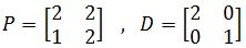
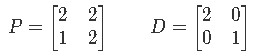
Let . Compute if:
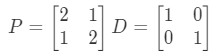
Equation for Example 1: Matrices P and D -
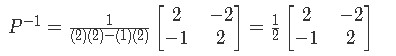
The first step in order to compute is to obtain the inverse of matrix P using equation 3.
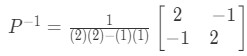
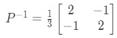
Equation for example 1(a): Inverse of matrix P -
Having all P, D and we just follow the process shown in equation 2 to obtain :


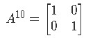
Equation for example 1(b): Matrix A elevated to the 10th power
This operation may now seem very simple but there is catch here, although we have provided P and D in for this example, they are usually not given in exam problems or assignments, you actually have to obtain them yourself. So, how exactly do we find P and D to work through the formula A= ? You need to follow the next steps:
- To find P:
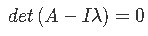
- Calculate the eigenvalues of A using the formula det
- Find the eigenvectors of each eigenvalue
- Use the eigenvectors as columns of matrix P
- To find D:
- Fill the diagonal entries with corresponding eigenvalues
- Fill the rest of the entries as zero
Consequently, let us work an example of this:
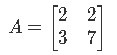
Example 2:
Diagonalize matrix A
Remember that diagonalizing means to find P, D and in the formula A= , therefore, let us find each of them following the steps we just described above.
We start by looking for P.
-
First, we have to calculate the eigenvalues of matrix A using the characteristic polynomial equation det , since the roots of the resulting characteristic polynomial are the eigenvalues of A.
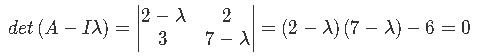
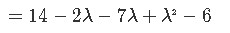
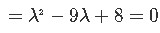
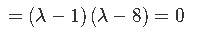
Equation for example 2(a): Finding eigenvalues -
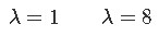
While working to find the eigenvalues , remember you can solve the quadratic equation with the quadratic formula. Having all the possible values of , let us find the eigenvectors associated with each of them. For =1:

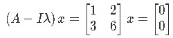
Equation for example 2(b): Finding an eigenvector associated to =1 (part 1) -
In order to solve for the vector we use an augmented matrix:
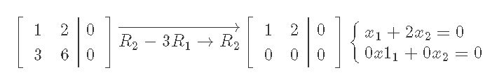
Equation for example 2(c): Finding an eigenvector associated to =1 (part 2) -
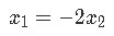
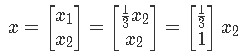
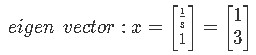
And so, we can write our general solution to obtain the eigenvector associated to =1.
Equation for example 2(d): Finding our eigen vector -
Following the same process, now to obtain the eigenvector associated to = 8:

Equation for example 2(e): Finding an eigenvector associated to = 8 (part 1) -
Using an augmented matrix to solve for vector :
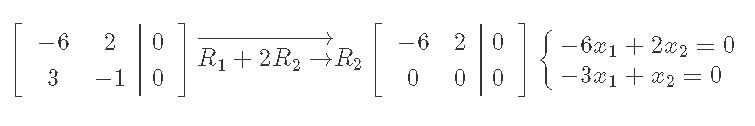

Equation for example 2(f): Finding an eigenvector associated to = 8 (part 2) -
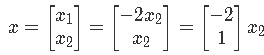
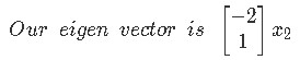
Writing the general solution and the final eigenvector associated to = 8
Equation for example 2(g): Finding an eigenvector associated to = 8 (part 3) -
Now we use the two eigenvectors found to write down P. Remember you just have to use the eigenvectors as columns to produce the matrix for P.

Equation for example2(h): Matrix P -
The next two things we have to write down are the matrices D and which at this point should come up straight forward. Since D is a diagonal matrix, we know the only nonzero components inside of it will be those in the main diagonal, thus, we fill the main diagonal using the eigenvalues found before of = 1 and = 8 in the next manner:
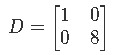
Equation for example 2(i): Diagonal matrix D -
Finally, we obtain the inverse of P by applying equation 3:
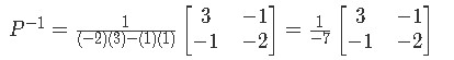
-
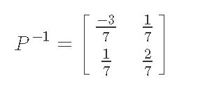
Equation for example 2(i): Equation for example 2(j): Matrix -
Remember what it means to have diagonalized a matrix, just obtaining the correct notations for D and , therefore, the complete diagonalization looks like:
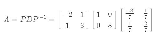
Equation for example 2(k): Diagonalization of matrix A
And that is how you diagonalize a matrix, you truly don't need to go through the process of calculating equation 1 because you would only end up with matrix A as a result, so the final result of the problems in this case is just for you to have found the values of D and .
Now, it is important that you know if a matrix is diagonalizable or not before you go through the trouble of calculating D and . In other words, imagine you go through the whole process we just described and computed above, just to realize you come up with trivial solutions? That is just a waste of time and energy in something that does not make any sense, and for that, we need to learn how to identify if a matrix is diagonalizable or not beforehand.
This verification process is what we call the Diagonalization theorem and is quite simple, you just need to check for two things:
- For an nxn matrix to be diagonalizable there should be n linearly independent eigenvectors.
This means that, if you have a 2x2 matrix, then you should be able to find 2 linearly independent eigenvectors for such matrix. If you have a 3x3 matrix, there should be 3 linearly independent eigenvectors and so forth.
- The condition AP = PD should be met.
After confirming the first condition, you must have already the values for the eigenvalues and eigenvectors, and so, use this information to come up with the matrices of P and D. Then multiply A times P and P times D in order to see if the result is equal.
If these two conditions are met for a given matrix A, then such matrix is diagonalizable. If you check for the first condition and is not met, then you can save yourself the trouble to go through the second condition since that is enough to tell you that the matrix you are provided with is not diagonalizable.
Let us work through an example problem in which you will have to identify if the given matrix is diagonalizable or not:
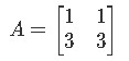
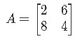
Example 3:
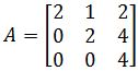
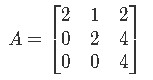
Is A diagonalizable?
To start the verification process through the diagonalization theorem, let us go through the first condition for matrix diagonalization: Are there two linearly independent eigenvectors? Let's find out!
-
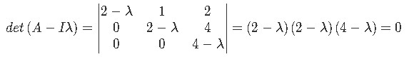
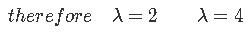
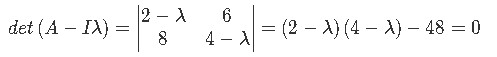
Remember we have to find the eigenvalues first:
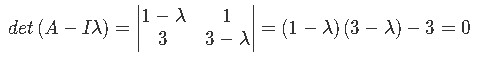
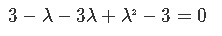

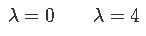
Equation for example 3(a): Finding the eigenvalues. -
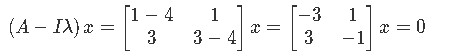
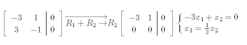
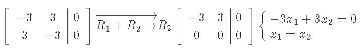
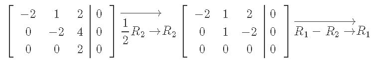
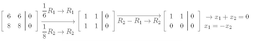
Now we find the associated eigenvectors. For = 0:

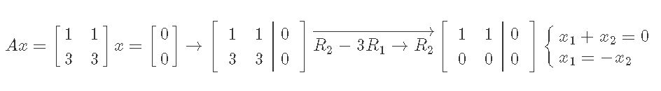
Equation for example 3(b): Finding the eigenvectors (part 1) -
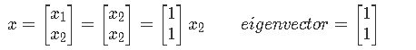
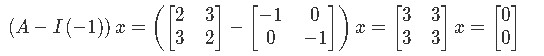
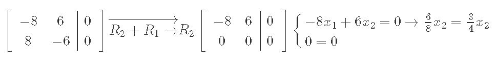
And for = 4:
Equation for example 3(c): Finding the eigenvectors (part 2) -
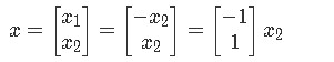
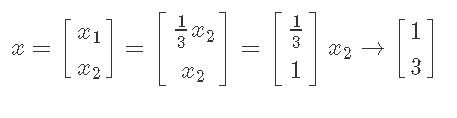
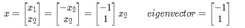
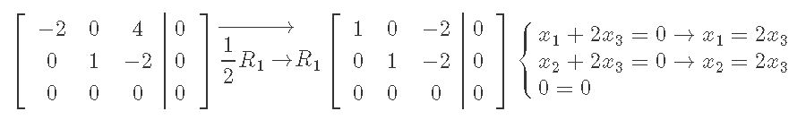
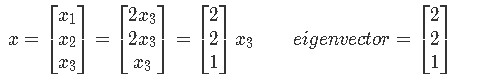
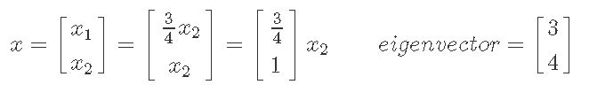
Therefore, the eigenvectors are:
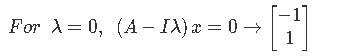
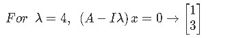
Equation for example 3(d): Finding the eigenvectors (part 3) -
By just observing the two eigenvectors, we can clearly see they are linearly independent. Therefore the first condition for diagonalization has been met.
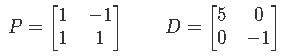
Let us now check if the equality AP = PD can be verified, for that, we need to write down matrices P and D. Remember, P is formed by combining the two eigenvectors (which are column vectors) into one matrix; D being a diagonal matrix is very simple because you just fill up the main diagonal spaces inside the appropriate square matrix using the obtained eigenvalues, while the rest of the digits in the matrix will be zero. And so, the matrices for P and D look as follows:
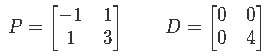
Equation for example 3(e): Matrices P and D -
The only step left is to compute the matrix multiplications AP and PD and check if the results are equal.
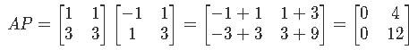
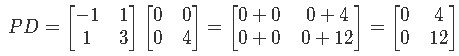

Equation for example 3(f): Verifying AP =PD
Further examples on diagonalization:
Example 4 takes on again in calculating a higher power of a given matrix, while examples 5 and 6 focus in finding out if the given matrix is diagonalizable. The lesson ends with example 7 which takes on the general way to diagonalize the matrix provided (which is just finding P, D and ).
Besides practicing with the examples we provide here, we do recommend visiting a few different sites to complement this lesson: A comprehensive example on the diagonalization of a matrix can be found there, and an interesting argument is made about the diagonalization of matrices and its theorem on this lecture piece.
For now, without further ado, let us work in our remaining examples:
Example 4:
-
Let A = P, D and ), then compute if:
Equation for example 4: Matrix P and matrix D -
Using equation 2, the expression for is as follows:

Equation for example 4(a): Matrix A to the fourth power -
To solve such equation we first need to calculate the inverse of matrix P:
Equation for example 4(b): Inverse of matrix P -
Elevating D to the fourth power is quite simple, just elevate each of the values inside the matrix to the fourth power and you will obtain:
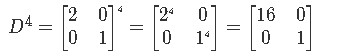
Equation for example 4(c): Diagonal matrix D to the 4th power -
Notice that in the case of matrices such as D, the power effect is noticeable only diagonally since the rest of the terms in the matrix are zeros. Therefore the rest of the terms remain as zeros, since zero to any power equals to zero.
Having all of the components ready, we can now compute :


Equation for example 4(d): Computation of A to the 4th power
Example 5:
Is the following matrix diagonalizable?
Using the theorem for diagonalization of a matrix, verify the two required conditions: First, are there two linearly independent eigenvectors? And second, is the condition AP = PD met?
-
In order to find the eigenvectors, we have to find the eigenvalues related to A by using the characteristic polynomial equation:
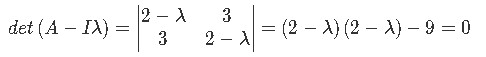
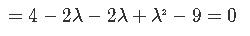


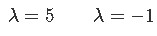
Equation for example 5(a): Finding the eigenvalues -
Then we have to find the associated eigenvector to each of the eigenvalues found. For = 5:
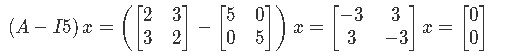
Equation for example 5(b): Finding an eigenvector associated to =5 (part 1) -
Using and augmented matrix to solve for the vector and obtain the associated eigenvector.
Equation for example 5(c): Finding an eigenvector associated to =5 (part 2) -
Now doing the same for = -1
Equation for example 5(d): Finding an eigenvector associated to = -1 (part 1) -
Working through the corresponding augmented matrix to obtain the second eigenvector:
Equation for example 5(e): Finding an eigenvector associated to = -1 (part 2) -
And so, we have two linearly independent eigenvectors and the first condition for matrix diagonalization has been met.
To continue, let us check for the second condition which says that the matrix multiplication AP must be equal to PD. For that, we write down the matrices P and D using the eigenvectors and eigenvalues found:
Equation for example 5(f): Matrices P and D -
Computing AP and PD and comparing them:


Equation for example 5(g): Confirming AP = PD
And so, the second condition is met and we can conclude that A is diagonalizable.
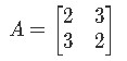
Example 5:
Can you diagonalize matrix A if A looks as follows:
To diagonalize A you need to check the two conditions of the diagonalization theorem. First, since A is a 3x3 matrix, are there 3 linearly independent eigenvectors?
-
We start by finding the eigenvalues:
Equation for example 6(a): Finding the eigenvalues -
Computing the eigenvector associated to = 2:
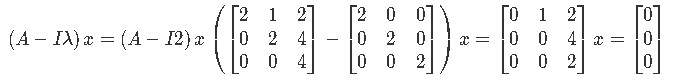
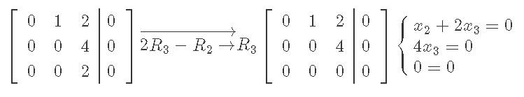
Equation for example 6(b): Finding an eigenvector associated to = 2 (part 1) -
Therefore, the components and are equal to zero, while the component is a free variable. Writing down the general solution and eigenvector associated to = 2 using the found components:
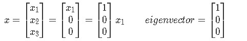
Equation for example 6(c): Finding an eigenvector associated to = 2 (part 2) -
Repeating this process to find the eigenvector associated to =4:
Equation for example 6(d): Finding an eigenvector associated to = 4 (part 1) -
Writing down the general solution and the eigenvector:
Equation for example 6(e): Finding an eigenvector associated to = 4 (part 2)
And so we run into a problem, through this method we can only find two linearly independent eigenvectors, which means that the very first condition for the theorem of a diagonalized matrix is not met. Therefore, our final conclusion is that for this problem, A is not a diagonalizable matrix.
Example 7:
Diagonalize the following matrix:
-
For this problem we just need to find P, D and . So let us start by computing P. We do so using the characteristic polynomial equation to find the appropriate eigenvalues and then their associated eigenvectors:


Equation for example 7(a): Finding the eigenvalues -
Next, we find the associated eigenvector to = 10:

Equation for example 7(b): Finding an eigenvector associated to = 10 (part 1) -
Writing the general solution for vector and the found eigenvector:
Equation for example 7(c): Finding an eigenvector associated to = 10 (part 2) -
Notice that since is a free variable which can take any value, we have made it equal to 4 in order to obtain a simplified eigenvector.
Now computing the associated eigenvector to = -4:

Equation for example 7(d): Finding an eigenvector associated to = -4 (part 1) - And we write down the general solution and obtained eigenvector:
Equation for example 7(e): Finding an eigenvector associated to = -4 (part 2) - Having found the eigenvalues and eigenvectors, we can now construct both P and D:
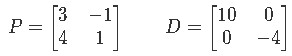
Equation for example 7(f): Matrix P and matrix D - Using P, we can now compute its inverse:
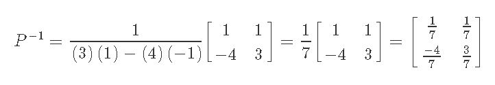
Equation for example 7(g): Inverse matrix of P - And our final solution is:

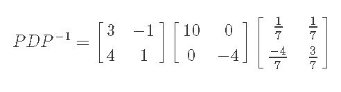
Equation for example 7(h): Final solution showing the components for the diagonalization of A And so, we have come to the end of our lesson on diagonalization matrix methods. Do not forget to visit the links provided whenever you need a review or want some more practice.
An matrix is diagonalizable if and only if has linearly independent eigenvectors.
If you have linearly independent eigenvectors, then you can use the formula
where:
The columns of are the eigenvectors
The diagonal entries of are eigenvalues corresponding to the eigenvectors
is the inverse of
To see if a matrix is diagonalizable, you need to verify two things
1. There are n linearly independent eigenvectors
2.
Useful fact: If is an matrix with distinct eigenvalues, then it is diagonalizable. - And we write down the general solution and obtained eigenvector: