Understanding Properties of Linear Transformations

Dive into the essential properties of linear transformations. Master additivity, homogeneity, and zero vector concepts. Enhance your linear algebra skills with clear explanations and practical examples.

Properties of linear transformation

What is a linear transformation

A transformation is a technique in which a vector gets converted into another by keeping a unique element from each of the original vector and assigning it into the resulting vector. This process basically maps one vector space into another. There may be different kinds of transformations in mathematics but the case of a linear transformation in linear algebra is that which preserves linear combinations from the original expression to the resulting one, in simple words, it preserves the way addition and scalar multiplication operate from the original vector to the transformed vector. A linear transformation example can also be called linear mapping since we are keeping the original elements from the original vector and just creating an image of it.

Recall the matrix equation Ax = b, normally, we say that the product of $A$ and $x$ gives $b$. Now we are going to say that $A$ is a linear transformation matrix that transforms a vector $x$ into a vector $b$ (we now call b an image of a linear transformation of $x$).


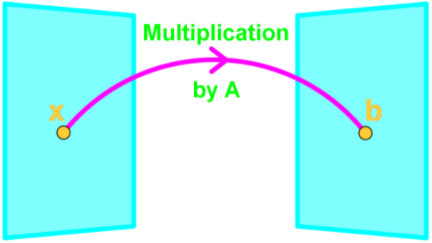
In a sense $A{x}$ is a function where if we plug in a vector, then it spits out another vector. If we call this function $T(x)$, then $T(x)=Ax$, where $T$ is the transformation. Note that $T(x)$ is an image of $x$ since $T(x)=b$;

How to do a linear transformation

From the linear transformation definition we have seen above, we can plainly say that to perform a linear transformation or to find the image of a vector $x$, is just a fancy way to say "compute $T(x)$".

So to compute a linear transformation is to find the image of a vector, and it can be any vector, therefore:

$T(x)$ = Image of $x$ under the transformation $T$

$T(v)$ = Image of $v$ under the transformation $T$

And so, if we define $T$: $R^{2} \,$→$\, R^{2}$ by $T(x)=Ax$. Find the image of $v$ under $T$ if:


So our goal is to find $T(v)=Av$
For that, remember our matrix multiplication guide:



And so, we perform the transformation:



Therefore the image of $v$ is:


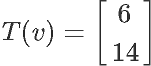
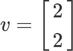
But what if the question gives the image and asks you to find the original vector? Let us use the same vectors as above and think how can we do the reverse engineering to obtain $v$, we start by working out the matrix equation below:


We use what we learned on the lesson about representing a linear system as a matrix, and write down an augmented matrix from our matrix equation above. Then in order to solve for vector v we just have to use row reduction and echelon forms!


And as you can see, we just got the linear transformation proof by reversing the process and obtaining the same vector v we started with:

Properties of Linear transformations

There are many linear transformation applications, but before start working on problems where we can use them, it is time to look into their properties. On our last lesson we talked about the image and the range of linear transformation $T(x)$, now let us see how the operations of addition/subtraction and multiplication apply to them.

Recall from last chapter the 2 properties of $Ax$:

1. $A(u+v) = Au + Av$
2. $A(cu) = c(Au)$

where u$u$ and v$v$ are vectors in $R^{n}$ and $c$ is a scalar.

Now the properties of linear transformations are very similar. Linear transformation preserves the operations of vector addition/subtraction and scalar multiplication. In other words, If $T$ is linear, then:

1. $T(u+v) = T(u) + T(v)$
2. $T(cu) = cT(u)$
3. $T (\rightharpoonup_{0}) = \rightharpoonup_{0}$

We can even combine property 1 and 2 to show that:

$T(cu \,+\, dv) = cT(u) \,+ \, dT(v)$
where $u$, $v$ are vectors and $c$, $d$ are scalars. Note that if this equation holds, then it must be linear.
What if you have more than 2 vectors and 2 scalars? What if you have p vectors and p scalars? Then we can generalize this equation and say that:

$T(c_{1}v_{1} \,+\, c_{2}v_{2} \, + \, . . . \, + \, c_{p}v_{p}) = c_{1}T(v_{1}) \,+ \, c_{2}T(v_{2}) \,+ \, . . . \, + \, c_{p}T(v_{p}) \,+ \,$
Notice that transformations of linear functions are distributive. And again if this equation holds, then it must be linear.

Example 1

Show that the transformation $T$ defined below is not linear: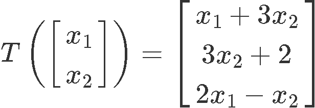


For this problem, we have to work with the matrix representation of linear transformation $T(x)$ to prove if the third property is held:


As you can see, the linear transformation does not result in a zero vector, and therefore, it cannot be linear.

Example 2

Show that the transformation T defined below is not linear:


This particular problem gets a little bit more complicated to prove since there is an absolute value inside the matrix of linear transformation $T$. Thus, we will use two properties instead of just one, we start with the first property to work through, and then the third property is used in combination while working on the left hand side of the first property to finish this problem:
We start by selecting our own vectors $u$ and $v$ (you can choose any vectors as long as the conditions are met).


And then using property one, we compute the transformations:


Notice in the left hand side we have used the third property too, to know the transformation of a zero vector is just the zero vector itself. Thus our result is:


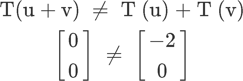
And since the first property is not met, the transformation is not linear.

Example 3

An affine transformation $T: R^{n} \,$→$\, R^{m} \,$ has the form $T(x)=Ax+b$, where $A$ is an $m \times n$ matrix of a linear transformation and $b$ is a vector in $R^{n}$. Show that the transformation $T$ is not a linear transformation when $b$ ≠ 0.

For this problem we need to check if any of the three properties of a linear transformation do not hold. Starting by the first property, we create the next table in which you can see how the left hand side and the right hand side of property one have been applied to the affine transformation above and see if they are equal when $b$ ≠ 0.

$T(u+v)$	$T(u)+T(v)$
$T(u+v)=A(u+v)\,+$ $b=Au+Av+b$	$T(u)+T(v)=(Au+b)\,+$ $(Av+b)=Au+Av+2b$

So as you can see, when $b$ ≠ 0. the first property of a linear transformation is not met, and that is it, it means this transformation T is not linear.

Example 4

Define $T: R^{n} \,$→$\, R^{m}$ to be a linear transformation, and let the set of vectors {$v_{1},v_{2},v_{3}$} be linearly dependent. Show that the set of vectors {$T(v_{1}),T(v_{2}),T(v_{3})$} are also linearly dependent.

This question may sound a little complicated, so let us bring back a quick review from our lesson on linear independence where we learnt that:

A set of vectors {$v_{1},v_{2},v_{3}, ... , v_{p}$} is said to be linearly independent if:

$v_{1}c_{1} + v_{2}c_{2} + v_{3}c_{3} + ... + v_{p}c_{p} = 0$
$iff: {c_{1} + c_{2} + c_{3} + ... + c_{p}} = 0$
So, linear independence produces a trivial solution, therefore in this case, since we are looking for a linearly dependant set of vectors, this means that we cannot have all zero solutions.

Thus, we are looking for $c_{1}T(v_{1}) + c_{2}T(v_{2}) + c_{3}T(v_{3}) = 0$ where ${c_{1}, c_{2}, c_{3}, ... , c_{p}}$ cannot all be zeros.

In order to show that the set of vectors ${T(v_{1}),T(v_{2}),T(v_{3})}$ are also linearly dependent, we will be using the three properties of linear transformations!

1. $T(u+v) = T(u) + T(v)$
2. $T(cu) = cT(u)$
3. $T (\rightharpoonup_{0}) = \rightharpoonup_{0}$

Therefore:
$v_{1}c_{1} + v_{2}c_{2} + v_{3}c_{3} = 0$
We replace this into the third property to obtain:

$T(0) = T(v_{1}c_{1} + v_{2}c_{2} + v_{3}c_{3}) = 0$
Now using the first property:

$T(v_{1}c_{1} + v_{2}c_{2} + v_{3}c_{3}) = T(v_{1}c_{1}) + T(v_{2}c_{2}) + T(v_{3}c_{3}) = 0$
And finally using the second property this becomes:

$T(v_{1}c_{1}) + T(v_{2}c_{2}) + T(v_{3}c_{3}) = c_{1}T(v_{1}) + c_{2}T(v_{2}) + c_{3}T(v_{3}) = 0$
So at this point we have arrived to exactly the formula we were looking for and now, we just have to show that ${c_{1}, c_{2}, c_{3}, ... , c_{p}}$ are not all zeros. The trick here is that since we already know from the beginning that the vectors ${v_{1},v_{2},v_{3}}$ are linearly dependent, by combining them as in the very first expression in equation 18 with ${c_{1}, c_{2}, c_{3}, ... , c_{p}}$ this makes them not all zero!, and so, we have made sure this particular characteristic applies to the whole expression found at the end of equation 18.

Hence: $c_{1}T(v_{1}) + c_{2}T(v_{2}) + c_{3}T(v_{3}) = 0$ is linearly dependant.

Example 5

Define $T: R^{n} \,$→$\, R^{m}$ to be a linear transformation and the set of vectors $v_{1} ,..., v_{p}$ are in $R^{n}$. In addition, let $T(v_{i}) = 0$ for $i = 1,2,..., p$. If $x$ is any vector in $R^{n}$, then show that $T(x) = 0$. In other words, show that $T$ is the zero transformation. If we have that:

$x = v_{1}c_{1} + v_{2}c_{2} + ...+ v_{p}c_{p}$
Computing the transformation of $x$:

$T(x) = T(v_{1}c_{1} + v_{2}c_{2} +...+ v_{p}c_{p}) = T(v_{1}c_{1}) + T(v_{2}c_{2}) +...+ T(v_{p}c_{p})$
$T(x) = c_{1}T(v_{1}) + c_{2}T(v_{2}) +...+ c_{p}T(v_{p})$

Using the condition provided in the problem $T(v_{i}) = 0$, this means that:

$T(v_{1}) = 0$
$T(v_{2}) = 0$
$\downarrow$
$T(v_{p}) = 0$
Then:

$T(x)=c_{1}T(v_{1})+c_{2}T(v_{2}) +... + c_{p}T(v_{p}) = c_{1}(0)+c_{2}(0) +...+ c_{p}(0) = 0$

And so, we just showed that $T(x) = 0$!

***
To continue your practice on linear transformations there are a few links we would like to recommend you such as this in depth calculus III lesson, of this article on linear transformations.

This finalizes our lesson for today, we hope you enjoyed it, see you in the next one!