Unlock the Power of Linear Equations in Real-World Applications

Discover how linear equations solve complex problems in economics, chemistry, and network analysis. Master practical skills for academic success and real-world problem-solving. Start your journey now!

Applications of linear systems

So far through our linear algebra course we have been looking into the methodology required while solving systems of linear equations with the use of notation of matrices. For the lesson of today, we will be talking about cases in which applying systems of linear equations is of benefit to resolve problems from varied distinct areas in life which, in our minds, we usually do not relate them much to the use of linear algebra.

But before we can go ahead and check into different applications of systems of linear equations in real life, we need to know how to solve a system of linear equations itself. In other words, let us take a quick review on the methods shown in the past few lessons.

How to solve systems of linear equations

For problems solving systems of linear equations in linear algebra, we usually use the method of Gaussian elimination (also named row reduction) to find the values of the variables involved in the system after we have converted such system into a matrix equation of augmented form.

If you remember from our lesson on solving a linear system with matrices using Gaussian elimination, the operations which can be applied to the rows of an augmented matrix in order to reduce it to an echelon form are:

1. Interchanging two rows
2. Multiplying a row by a constant (any constant which is not zero)
3. Adding a row to another row

One can also make combinations of these operations, and the resulting matrix, will be an equivalent simplified matrix which will allow us to see directly the value of each variable in the system. This final matrix is what we call the reduced row echelon form of the initial augmented matrix coming from a system of linear equations.

In our lesson on row reduction and echelon forms we saw the algorithm that needs to be followed to in order to arrive to the reduced echelon form of a matrix:

1. Look for the leftmost non-zero column. This is our pivot column
2. Find a non-zero entry in the pivot column. This is our pivot position. It should be at the very top of the pivot column.
3. Use matrix row reduction to make all the entries below the pivot equal to zero.
4. Ignore the row with the pivot and now operate on the next one to the right. Repeat Step 1-3 again and again until you have worked through all of the columns.
5. Find your rightmost pivot. Row reduce it until is equal to 1.
6. Make all the entries above this pivot equal to 0.
7. Repeat steps 5 and 6 for all the pivots in the reduced matrix.

Once the matrix in reduced echelon form, each row of such matrix will provide the final expression (or value) for the variable corresponding to each column on the matrix.

Such methods have been extensively explained in the past lessons, so we recommend that if you still have a few doubts, you can go back and have a review (as a suggestion of the lessons you will be required to know for this one, you can go ahead and check all of the links we have provided through this reading).

Applications of systems of linear equations

On this section we will be looking at real-life problems involving linear algebra. The three types of real-life applications we will be looking at are:

1. Linear systems in Economics
2. Linear systems with Chemical Equations
3. Linear systems with Network Flow

Let us then jump in directly into solving examples of each area, remember: Our goal is to make all of these questions into a matrix and then solve.

A country's economy is usually divided into sectors, a few that come to mind might be: manufacturing, services, energy and fuel, transportation, and other public or private sectors. Each of these sectors has a total output (which we will measure in dollars) for one year. This total output is the total amount of earnings for a year and is represented by the letter p, this particular revenue is then used, some or all of it may be invested by exchanging or buying from the other sectors in the economy.

For all of this trade, there must exist an equilibrium price where each sector has:

Income = expenses (expenditures)
Which means that the total amount of income in a sector must be equal to the total amount of expenses, or in other words, the total amount of income is the most that a sector can spend either buying, trading, or even keeping its own capital.
In economics, we can use linear algebra to determine the equilibrium price of outputs for each sector, take a look at the two examples below:

Example 1

Assume that the economy has 2 sectors: Transportation and Manufacturing.

• Transportation sells 60% of its output to Manufacturing and keeps the rest of the output.
• Manufacturing sells 80% of its output to Transportation and keeps the rest.

Create an exchange table for this economy, and find the set of equilibrium prices.


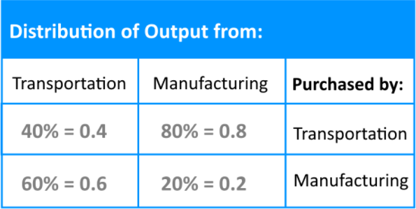
On this exchange table, what you can see in the first two columns are the total outputs measured in dollars for one year for each of the two economic sectors given, in other words, this was their income for their year and how they put it out for others to buy. Notice the quantities have been rewritten down from the percentages provided to their equivalency in decimal notation. The rows for the table represent the expense each sector went through.

Since total output is usually defined as $P$, we call the first column $P_{t}$ (for total output from transportation) and the second $P_{m}$ (for total output from manufacturing) and following the principle of income = expenses we can form the next equations:

0.4$P_{t} \, + \,$0.8$P_{m} = P_{t}$ 0.6$P_{t} \, + \,$0.2$P_{m} = P_{m}$
Where the left hand side of each equation represents the income and the right hand side represents the expenses of each economic sector.
Now, since we will be solving this system of equations through matrix notation, we need to convert the system to an augmented matrix, but before we can do that, we need to pass all of the unknown variables ($P_{t}$ and $P_{m}$) to the left side of the equations:

0.4$P_{t} \, + \,$0.8$P_{m} = P_{t} \,$→$\, -$0.6$P_{t} \, + \,$0.8$P_{m} = 0$ 0.6$P_{t} \, + \,$0.2$P_{m} = P_{m} \,$→$\, -$0.6$P_{t} \, - \,$0.8$P_{m} = 0$
We construct the augmented matrix and row reduce it to solve for the unknown variables:


As you can see, $P_{m}$ is a free variable since there is no corresponding pivot for it on the augmented matrix, and so out solutions in parametric form are:


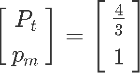
The set of equilibrium prices can be obtained by setting the free variable $P_{m} =$1, therefore:

Example 2

Assume that the economy has 3 sectors: Manufacturing, Services, and Extraction.

• Manufacturing sells 50% of its output to Services, and 50% to Extraction.
• Services sells 30% of its output to Manufacturing, 60% to extraction, and keeps the rest.
• Extraction sells 80% of its output to manufacturing, 10% to services, and keeps the rest.

Find a set of equilibrium prices for when the extraction output is 80 units.


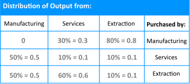
Following the same methodology we used in our last problem, we obtain the system of linear equations from the exchange table and move all of the unknowns variables to the left hand side.

0.3$P_{s} \, + \,$0.8$P_{\epsilon} = P_{m} \,$→$\, - \, P_{m} \, +\,$0.3$P_{s} \, + \,$0.8$P_{\epsilon} = 0$
0.5$P_{m} \, + \,$0.1$P_{s} \, + \,$0.1$P_{\epsilon} = P_{s} \,$→$\,$0.5$P_{m} \, - \,$0.9$P_{s} \, + \,$0.1$P_{\epsilon} = 0$
0.5$P_{m} \, + \,$0.6$P_{s} \, + \,$0.1$P_{\epsilon} = P_{\epsilon} \,$→$\,$0.5$P_{m} \, + \,$0.6$P_{s} \, - \,$0.9$P_{\epsilon} = 0$
We construct the augmented matrix and row reduce it to solve for the unknown variables:





As you can see, $P_{\epsilon}$ is a free variable since there is no corresponding pivot for it on the augmented matrix, and so out solutions in parametric form are:


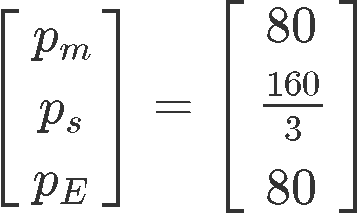
For this particular problem, it is asked to find the set of equilibrium prices when $P_{\epsilon} = 80$ and so:



In Chemistry, we can use linear algebra to balance chemical equations. Take a look at the next exercise to see the process:

Example 3

Having the next chemical reaction equation

$N_{2} + H_{2} \,$→$\, NH_{3}$
How do we balance a chemical equation? We use coefficients! The coefficients will allow us to find out the quantity needed of the molecules in the left hand side of the reaction, that would proportionally produce a certain amount of the compound in the right hand side of the reaction. Truly if you think about it, a chemical reaction equation can be looked as an algebraic expression too, where the variables would be the name of the elements, or molecules of compounds you are using throughout the reaction. In here,we have inputted coefficients inside parenthesis to balance equation 10:

$(x_{1}) + N_{2} \, + \, (x_{2}) + H_{2} \,$→$\, (x_{3}) + NH_{3}$
How do we create a matrix and solve for the variables? This can be a little tricky, but for each element, element molecule or compound found in the chemical reaction, we construct a vector which lists the number of atoms of each reactant. Look how this is done for the reaction above:


Such column vectors can then be used to create the proper matrix to find the correct values for $x_{1}$, $x_{2}$ and $x_{3}$ which will balance the reaction equation. Thus, having the vectors above we obtain:


Notice how in the very right hand side we have a vector equation similar to those seen on our lesson about linear combinations and vector equations. We know that we can convert such equation into an augmented matrix, which we can later solve using the three types of matrix row operations through Gaussian elimination. But before we do that, we have to put all of the variables in the left hand side of the equation, so out vector equation is now:


And so, the augmented matrix looks as follows:


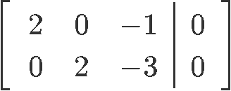
Using row reduction to obtain the value for each of the unknown variables corresponding to the matrix we obtain:



Where we can clearly see that $x_{3}$ is a free variable. Thus the solutions in parametric form are:


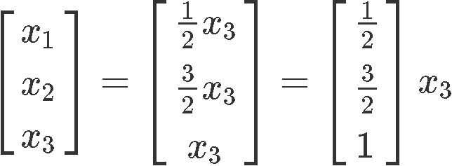
Now, there is something important to consider in here: these cannot be our final solutions because these variables represent the coefficients of reactants in a chemical reaction equation, and thus, they MUST be full numbers (you cannot divide either atoms or molecules without changing their properties, and so, these need to be full numbers). And so, since $x_{3}$ is a free variable, we can set it up to any value we want without changing the proportion within the variables. And so, we set $x_{3} = 2$ since is the smallest value it can have to produce full numbers as values for the rest of the variables. Thus:


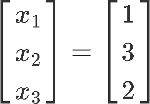
So our balanced chemical reaction equation is:

$N_{2} \, + \, 3H_{2} \,$→$\, 2NH_{3}$
In summary, we balanced by counting the number of elements in a compound, and turning each coefficient as a variable to solve. Let us work through another example of this below.

Example 4

Having the next chemical reaction equation:

$Na_{3} PO_{4} \, + \, MgCl_{2} \;$→$\; NaCl \, + \, Mg_{3} (PO_{4})_{2}$
We input the unknown coefficients to be solved for:

$(x_{1})Na_{3} PO_{4} \, + \, (x_{2})MgCl_{2} \;$→$\; (x_{3})NaCl \, + \, (x_{4})Mg_{3} (PO_{4})_{2}$
In order to write down the column vectors representing the number of atoms from each element involved, we first have to identify all of the type of elements that appear in the reaction equation. We have written the list as a column vector (to serve as template for each reactant vector) as is shown below:


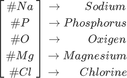
And so, the column vector for each reactant is:


Putting all of these vectors into a column vector equation we obtain the expressions below.


And transcribing these vector equations into an augmented matrix we obtain:


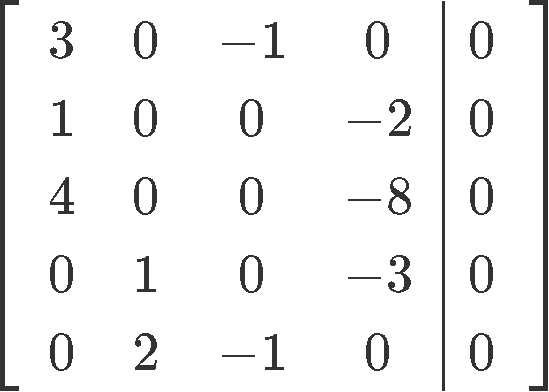
Now let us row reduce this matrix into its reduced echelon form so we can find the value for each unknown:






And so our final solution in parametric form can be seen as:


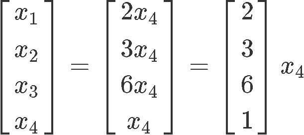
Notice that $x_{4}$ is a free variable, and so, we can set it up to any value we want! The simplest value to choose for the free variable is to just make it equal to one:


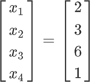
And the final chemical reaction equation is:

2$Na_{3}PO_{4} \, + \, 3MgCl_{2} \,$→$\,$6$NaCl \, + \, Mg_{3}(PO_{4})_{2}$
Network flow refers to a connected system, named the network, which has elements going in and going out (thus the term flow). A network in itself has a set of points called nodes which are the connections in a set of branches. In this way, each branch has a flow direction pointing to a node, and each node has flow in and flow out, meaning the elements traveling through the network will be passing through each node and the same amount of elements that arrive to each of them are the same ones that get out and go away (there are no losses).
And so, we can use linear algebra to study the flow of some quantity through a network. Just keep in mind the rule for the nodes:

Flow in = Flow out

Example 5

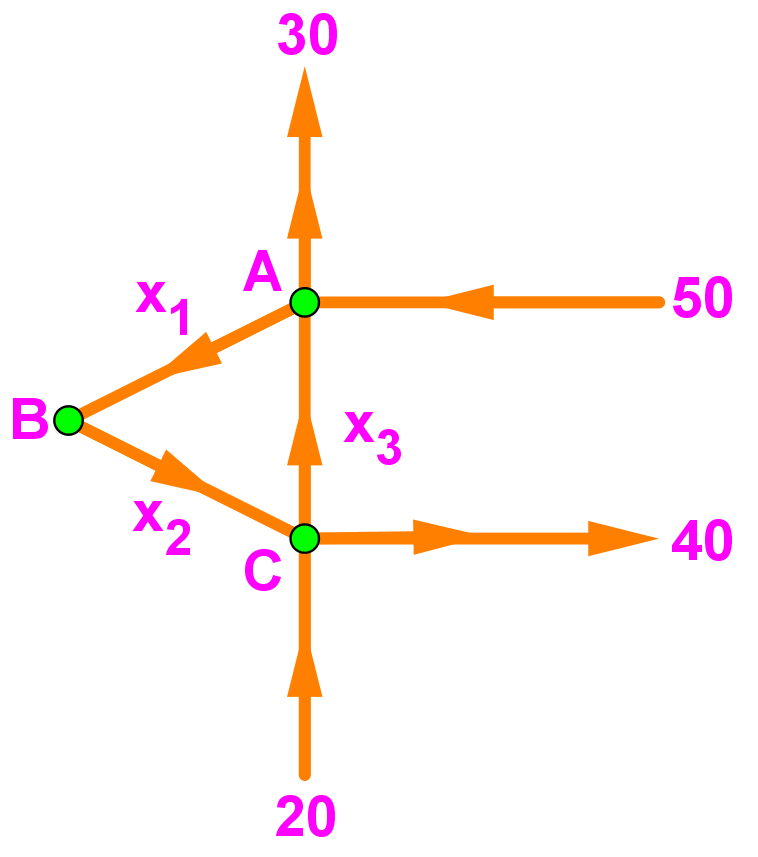
Find the general solution of the network flow. Assuming that all flows are non negative, what is the minimum value of 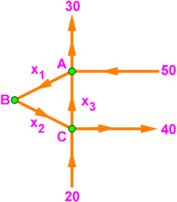$x_{1}$ and $x_{2}$?


On this example we have three nodes, in order to obtain the equations related to the flow at each of them we first construct the next table with the elements that will be needed:


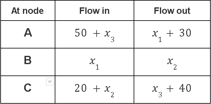
Which brings about the equations:

50$\, + \, x_{3} = x_{1} \, + \,$30$\,$→$\, x_{1} \, - \, x_{3} = \text(20)$ $x_{1} = x_{2} \,$→$\, x_{1} \, - \, x_{2} = \text(0)$ 20$\, + \, x_{2} = x_{3} \, + \,$40$\,$→$\, x_{2} \, - \, x_{3} = \text(20)$
Above we have written down the equations coming from the table, and we have put all of the unknown variables to the left hand side of each equation so we can convert the system into the next augmented matrix:


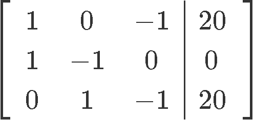
Row reducing the equation in order to find the values for $x_{1}$, $x_{2}$ and $x_{3}$:




And so we have that the values of $x_{1}$ and $x_{2}$ are:

$x_{1} = x_{3} \, + \,$20 $x_{2} = x_{3} \, + \,$20 $x_{3} = x_{3}$
In order to obtain their minimum possible value we can set the free variable $x_{3}$ to our most convenient value for that purpose, in other words, let us choose $x_{3}$!
For that, remember flow cannot have negative elements going into a node, but we can have zero elements going in (basically nothing going in, if you think about it, a negative value would actually mean the elements are going out and since these elements are in the other side of the equation they cannot be taken as negatives). And so, the smallest possible value of $x_{3}$ is zero, therefore, the minimum values of $x_{1}$ and $x_{2}$ are:

$x_{1} =$20$\,$ and $\, x_{2} =$20
And that is our final answer!

***
For even more examples on the applications of systems of equations we recommend you to take a look at these algebra notes, remember that as long as you have a linear system, you can convert it into matrix equations to solve. Also, a very interesting and modern application of linear systems can be studied on this innovating scientific paper published a few years ago about solving systems of linear equations on a quantum computer note how the possibilities are endless when knowing math!

We hope you have enjoyed the lesson of today, see you in the next one!