Mastering Applications of Linear Models in Economics
Dive into the world of linear models and their applications in economics. Learn powerful regression techniques, analyze real-world data, and gain insights for informed economic decision-making and policy formulation.

  1. Intros0/4 watched
  2. Examples0/5 watched
  1. 0/4
  2. 0/5
Now Playing:Application to linear models – Example 0a
Intros
0/4 watched
  1. Applications to Linear Models Overview:
  2. Applications to Linear Models Overview:
    Applying Least-Squares Problem to Economics
    • Go from Ax=bAx=b to Xβ=yX\beta=y
    XX → design matrix
    β\beta → parameter vector
    yy → observation vector
  3. Applications to Linear Models Overview:
    Least-Squares Line
    • Finding the best fit line
    • Turning a system of equations into Xβ=yX\beta =y
    • Using the normal equation XTXβ=XTyX^T X\beta=X^T y
    • Introduction of the residual vector
Examples
0/5 watched
  1. Finding the Least-Squares Line
    Find the equation y=β0+β1xy=\beta_0+\beta_1 x of the least-squares line that best fits the given data points:
    (0,1),(1,2),(2,3),(3,3)(0,1),(1,2),(2,3),(3,3)
    Inner product, length, and orthogonality
    Notes
    In this section, we will apply least square problems to economics.

    Instead of finding the least squares solution of Ax=bAx=b, we will be finding it for Xβ=yX\beta =y where

    XX → design matrix
    β\beta → parameter vector
    yy → observation vector

    Least-Squares Line
    Suppose we are given data points, and we want to find a line that best fits the data points. Let the best fit line be the linear equation
    y=β0+β1xy=\beta_0 + \beta_1 x

    And let the data points be (x1,y1),(x2,y2),,,(xn,yn)(x_1,y_1 ),(x_2,y_2 ),\cdots,,(x_n,y_n ). The graph should look something like this:
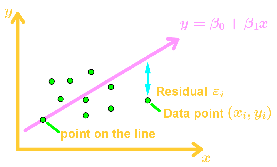
    best fit liney=beta_0 + beta_1 x

    Our goal is to determine the parameters β0\beta_0 and β1\beta_1. Let's say that each data point is on the line. Then
    best fit line data points beta_0 + beta_1 x

    This is a linear system which we can write this as:
    linear system

    Then the least squares solution to Xβ=yX\beta=y will be XTXβ=XTyX^T X \beta =X^T y.

    General Linear Model
    Since the data points are not actually on the line, then there are residual values. Those are also known as errors. So we introduce a vector called the residual vector ϵ\epsilon, where
    ϵ=yXβ\epsilon = y - X\beta
    y=Xβ+ϵ y = X\beta + \epsilon

    Our goal is to minimize the length of ϵ\epsilon (the error), so that XβX\beta is approximately equal to yy. This means we are finding a least-squares solution of y=Xβy=X\beta using XTXβ=XTyX^T X\beta=X^T y.

    Least-Squares of Other Curves
    Let the data points be (x1,y1),(x2,y2),,,(xn,yn)(x_1,y_1 ),(x_2,y_2 ),\cdots,,(x_n,y_n ) and we want to find the best fit using the function y=β0+β1x+β2x2y=\beta_0+\beta_1 x+\beta_2 x^2, where β0,β1,β2\beta_0,\beta_1,\beta_2 are parameters. Technically we are using a best fit quadratic function instead of a line now.
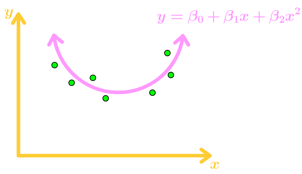
    best fit quadratic function

    Again, the data points don't actually lie on the function, so we add residue values ϵ1,ϵ2,,ϵn\epsilon_1,\epsilon_2,\cdots,\epsilon_n where

    add residue values 
 to data points

    Since we are minimizing the length of ϵ\epsilon, then we can find the least-squares solution β\beta using XTXβ=XTyX^T X\beta=X^T y. This can also be applied to other functions.

    Multiple Regression
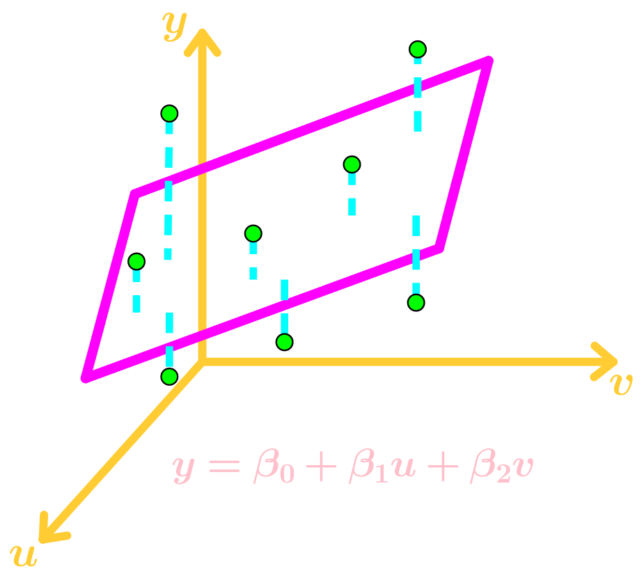
    Let the data points be (u1,v1,y1),(u2,v2,y2),,,(un,vn,yn)(u_1,v_1,y_1 ),(u_2,v_2,y_2 ),\cdots,,(u_n,v_n,y_n ) and we want to use the best fit function y=β0+β1u+β2vy=\beta_0+\beta_1 u+\beta_2 v, where β0,β1,β2\beta_0,\beta_1,\beta_2 are parameters.
    best fit function Multiple Regression

    Again, the data points don't actually lie on the function, so we add residue values ϵ1,ϵ2,,ϵn\epsilon_1,\epsilon_2,\cdots,\epsilon_n where

    add residue values to data points of the function

    Since we are minimizing the length of ϵ\epsilon, then we can find the least-squares solution β\beta using XTXβ=XTyX^T X\beta=X^T y. This can also be applied to other multi-variable functions.
    Concept

    Introduction to Applications of Linear Models

    Linear models play a crucial role in economics, offering powerful tools for analyzing and predicting economic phenomena. The introduction video provides an essential foundation for understanding these applications, bridging the gap between theoretical concepts and real-world scenarios. As we transition from abstract least squares problems to practical applications, we discover how linear models illuminate various economic relationships. These models are instrumental in forecasting economic trends, evaluating policy impacts, and understanding market dynamics. Economists utilize linear regression to examine factors influencing GDP growth, employment rates, and consumer behavior. In finance, linear models help assess risk and return relationships in portfolio management. The versatility of these models extends to analyzing supply and demand curves, estimating production functions, and studying international trade patterns. By mastering the application of linear models in economics, researchers and practitioners gain valuable insights into complex economic systems, enabling more informed decision-making and policy formulation.

    Example

    Applying Least-Squares Problem to Economics
    Go from Ax=bAx=b to Xβ=yX\beta=y
    XX → design matrix
    β\beta → parameter vector
    yy → observation vector

    Step 1: Introduction to Applications to Linear Models

    Welcome to the section on Applications to Linear Models. In this section, we will explore how to apply least-squares problems to real-life situations, particularly in the field of economics. If you are unfamiliar with least-squares problems, it is recommended to review the previous section as it provides essential background information.

    Step 2: Understanding Least-Squares Problems

    Least-squares problems involve finding the best approximated solution for the equation Ax=bAx = b. This method is used when the equation Ax=bAx = b has no exact solution, and we need to approximate a solution. The approximated solution obtained through this method is known as the least-squares solution.

    Step 3: Transitioning to Economics Notation

    To apply least-squares problems to economics, we need to adjust our notation. Instead of using the matrix equation Ax=bAx = b, we will use Xβ=yX\beta = y. This change in notation is standard in economics, although the underlying principles remain the same. Here, XX represents the design matrix, β\beta represents the parameter vector, and yy represents the observation vector.

    Step 4: Defining the Design Matrix

    In the context of economics, the design matrix XX is analogous to the matrix AA in the original equation. The design matrix contains the independent variables or predictors used in the model. When asked to find the design matrix, you are essentially identifying the matrix XX.

    Step 5: Understanding the Parameter Vector

    The parameter vector β\beta in economics corresponds to the solution vector xx in the original equation. The parameter vector contains the coefficients or parameters that we aim to estimate using the least-squares solution. These parameters are crucial for making predictions and understanding the relationships between variables in the model.

    Step 6: Identifying the Observation Vector

    The observation vector yy represents the dependent variable or the observed outcomes in the model. It is analogous to the vector bb in the original equation. The observation vector contains the actual data points that we use to fit the model and estimate the parameters.

    Step 7: Applying Least-Squares Solutions in Economics

    Now that we have defined the design matrix, parameter vector, and observation vector, we can apply the least-squares solution to estimate the parameters in the model. The goal is to find the parameter vector β\beta that minimizes the sum of the squared differences between the observed values yy and the predicted values XβX\beta. This process involves solving the normal equations or using matrix operations to obtain the least-squares estimates.

    Step 8: Practical Implications and Applications

    Understanding and applying least-squares problems in economics has significant practical implications. It allows economists to build models that can predict economic outcomes, analyze relationships between variables, and make informed decisions based on data. By accurately estimating the parameters, economists can gain insights into various economic phenomena and develop strategies to address real-world challenges.

    Step 9: Conclusion

    In conclusion, applying least-squares problems to economics involves transitioning from the notation Ax=bAx = b to Xβ=yX\beta = y. The design matrix XX, parameter vector β\beta, and observation vector yy play crucial roles in this process. By understanding these components and using the least-squares solution, we can build robust economic models and make data-driven decisions.

    FAQs

    Q1: What is the difference between simple linear regression and multiple regression in economics?
    A1: Simple linear regression involves one independent variable and one dependent variable, while multiple regression includes two or more independent variables. In economics, simple regression might analyze how income affects spending, while multiple regression could examine how income, age, and education level collectively influence spending patterns.

    Q2: How does the least squares method work in economic modeling?
    A2: The least squares method minimizes the sum of squared differences between observed data points and predicted values. In economic modeling, it's used to find the best-fitting line or plane that represents the relationship between variables. This method helps economists estimate parameters in regression models, allowing for accurate predictions and analysis of economic relationships.

    Q3: What are some common challenges in applying linear models to economic data?
    A3: Common challenges include multicollinearity (high correlation between independent variables), heteroscedasticity (non-constant variance of errors), omitted variable bias, and non-linear relationships. These issues can lead to inaccurate estimates and unreliable predictions. Economists must carefully test for these problems and use appropriate techniques to address them, such as robust regression methods or non-linear transformations.

    Q4: How are non-linear functions used in economic modeling?
    A4: Non-linear functions, such as quadratic or cubic models, are used when economic relationships don't follow a straight line. For example, the relationship between a worker's age and productivity might be modeled using a quadratic function to capture an initial increase followed by a decline. These models allow economists to represent more complex economic phenomena that simple linear models can't adequately describe.

    Q5: What software tools are commonly used for economic modeling and regression analysis?
    A5: Popular software tools for economic modeling include R, Stata, SPSS, and EViews. R is an open-source platform with extensive statistical capabilities. Stata is widely used in academia and offers powerful data management features. SPSS is user-friendly and commonly used in social sciences. EViews specializes in time-series analysis and econometric modeling. The choice of software often depends on the specific requirements of the economic analysis and personal preference.

    Prerequisites

    Understanding the application of linear models is a crucial skill in various fields, including statistics, economics, and data science. To fully grasp this concept, it's essential to have a solid foundation in several prerequisite topics. These topics provide the necessary background knowledge and skills to effectively apply linear models in real-world scenarios.

    One of the fundamental prerequisites is regression analysis. This statistical method is at the core of many linear modeling techniques. Regression analysis helps us understand the relationships between variables and make predictions based on these relationships. A key aspect of regression analysis is understanding residuals, which are the differences between observed and predicted values. Mastering the concept of residuals in regression analysis is crucial for assessing the fit and accuracy of linear models.

    Another critical prerequisite is the matrix equation Ax=b. This concept from linear algebra forms the mathematical foundation for many linear modeling techniques. Understanding how to solve and interpret matrix equations is essential when working with systems of linear equations, which are often encountered in complex linear models. The ability to manipulate and solve matrix equations efficiently can greatly enhance your capacity to work with advanced linear modeling techniques.

    Additionally, familiarity with the characteristics of quadratic functions is important for applications to linear models. While linear models primarily deal with straight-line relationships, understanding quadratic functions can be beneficial in several ways. For instance, in econometrics, quadratic functions are often used to model non-linear relationships or to capture diminishing returns. Knowledge of how these functions behave and their unique properties can help in interpreting more complex models and understanding when linear approximations may or may not be appropriate.

    By mastering these prerequisite topics, students can develop a more comprehensive understanding of linear models and their applications. Regression analysis provides the statistical framework for model building and evaluation. The matrix equation Ax=b offers the mathematical tools for solving complex systems of equations often encountered in multivariate linear models. And understanding quadratic functions can help in recognizing the limitations of linear models and when more complex functional forms might be necessary.

    As you delve into the application of linear models, you'll find that these prerequisite topics are not just abstract concepts but practical tools that you'll use repeatedly. They form the building blocks upon which more advanced concepts are constructed. By investing time in thoroughly understanding these prerequisites, you'll be better equipped to tackle complex problems, interpret results accurately, and apply linear models effectively in various real-world situations.