Least-squares problem

Least-squares problem

Method of least squares

In linear algebra, we have talked about the matrix equation Ax=b and the unique solutions that can be obtained for the vector $x$, but, sometimes $Ax=b$ does not have a solution, and so, for those cases our best approach is to approximate as much as possible a value for $x$.
Therefore, the topic for the lesson of today is a technique dedicated to obtain that close-enough solution. The technique has been called least-squares and is based on the principle that since we cannot obtain the solution of the vector $x$ for the matrix equation $Ax=b$, then we have to find an $x$ that produces a multiplication $Ax$ as close as possible to the vector $b$

If $A$ is an $m \times n$ matrix and $b$ is a vector in $R^n$, then the least-squares solution for $Ax=b$ is the vector $x$in $R^n$ where the following condition applies for all $x$ in $R^n$:

$\parallel b- A\hat{x}\parallel\ \; \leq \; \, \parallel b-Ax\parallel$
This means that if we cannot obtain a solution for the equation $Ax=b$, then our best approximation to the true value of $x$, which we call $x$ or the least-squares solution (also called the least squares approximation), can be obtained if the condition in equation 1 is met. The left hand side on this equation is what we call the magnitude of the smallest possible error of the best approximation to the vector $x$, in other words, is the smallest possible error in $x$. The right hand side is the smallest possible error in $x$.

Having seen how the method of least squares is related to errors, we can talk about how this relates to a real life scenario. Basically, the idea of the least square method is that as much as we want to be accurate while performing measurements during studies or experiments, the truth is that there is just so much precision we can obtain as humans with non-perfect tools in a non-perfect world. From the scale of the measurements, to random changes in the environment, etc. There will be scenarios in which our measurements are not good enough and for that we have to come up with a solution that approximates as much as possible to the true value of the element we are measuring. This is where the least-squares solution brings a way to find a value that otherwise is unattainable (and actually, this is just the best approximation we can have but not the real value itself).

Least squares solution

Having a $m \times n$ matrix $A$ and column vector $b$ in $R^n$, using the next matrix equation for the relationship of the unit vector $x$ and the matrix $A$ and its transpose:

$A^TA\hat{x} = A^Tb$
We can solve for the unit vector $\hat{x}$ and we have that:

$\hat{x} = (A^TA)^{-1}A^Tb$
This is what is called the least-squares solution of a matrix equation $Ax=b$

The steps to obtain the least-squares solution $\hat{x}$ for a problem where you are provided with the matrix $A$ and the vector $b$ are as follows:

1. If you follow the matrix equation found in equation 2:
1. Find the transpose of vector $A: A^T$
2. Multiply $A^T$ times matrix $A$, to obtain a new matrix: $A^TA$
3. Multiply the transpose of matrix $A$ with the vector $b$
4. Construct the matrix equation $A^TA \hat{x}=A^Tb$ using the results from steps b and c
5. Transform the matrix equation above into an augmented matrix
6. Row reduce the augmented matrix into its echelon form to find the components of vector $\hat{x}$
7. Construct the least squares solution $\hat{x}$ with the components found.


2. If you follow the formula for $\hat{x} \,$ that is found in equation 3:
1. Start by obtaining the transpose of matrix $A: A^T$
2. Multiply $A^T$ times matrix $A$, to obtain a new matrix: $A^TA$
3. Find the inverse of matrix $A^TA$
4. Multiply the transpose of matrix $A$ with the vector $b$
5. Multiply the results you obtained in steps 4 and 5 together to obtain: $\hat{x} =(A^TA)^{-1} A^Tb$

There are also some alternative calculations in order to find the least-square solution of a matrix equation. For example: let A be a mxn matrix where $a_1,a_2,...,a_n$ are the columns of $A$. If $Col(A)=${$a_1,a_2,...,a_n$} form an orthogonal set (meaning that all the columns inside matrix $A$ are orthogonal to each other), then we can find the least-squares solutions using the equation:

$A\hat{x} = \hat{b}$
Where we have that $\hat{b}$ encompases the orthogonal projection of b onto the columns of $A$:

$\hat{b} =$proj$_{Col(A)}b = \frac{b\cdot a_1}{a_1 \cdot a_1}a_1 \; + ... \; + \frac{b\cdot a_n}{a_n \cdot a_n}a_n$
Before we continue onto the next section, let us focus for a moment in what is called the least-squares error: Remember in the first section we called the left hand side of equation 1 as the magnitude of the smallest possible error of the best approximation to the vector $x$, in other words, the magnitude of the smallest possible error in $\hat{x}$. This part of equation one is what is called the least-squares error:

$\parallel b- A\hat{x}\parallel$

Solving least squares problems

During the next exercises we will take a look at different examples on the method of least squares. Make sure you follow all of the operations and if in doubt, do not hesitate to message us!

Example 1

Given $A$ and $b$ as shown below, find a least squares estimate solution for equation 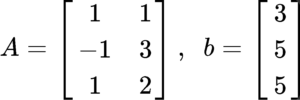$Ax=b$.


This problem is asking to solve for $\hat{x}$ using the least squares formula as defined in equation 3, and so, we must follow the steps we have described before. The first thing to do is to obtain the transpose of matrix $A$. Remember that the transpose of a matrix is obtained by swapping the elements that used to form the rows in the original matrix as the columns in the transform, and so, we swap rows to columns and columns to rows to find $A^T$:


Then we multiply the matrix obtaining through the transpose in equation 8 with matrix $A$, and so, $A^TA$ goes as follows:


Now we find the inverse of matrix $A^TA$:


On the other hand, now we multiply the transpose of matrix $A$, found in equation 8, with the vector $b$:


Now we can finally obtain $\hat{x}$ by multiplying the results found in equations 10 and 11: $\hat{x}=(A^TA)^{-1} A^Tb$

Example 2

Describe all least square solutions of equation $Ax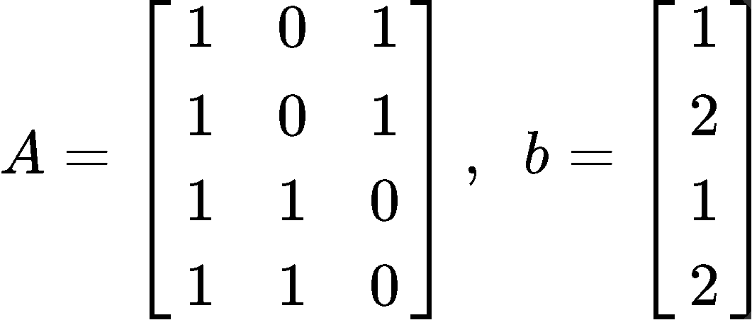=b$ if:


Now following the steps to solve for $\hat{x}$ using the least squares equation 2: $A^TA\hat{x}=A^Tb$
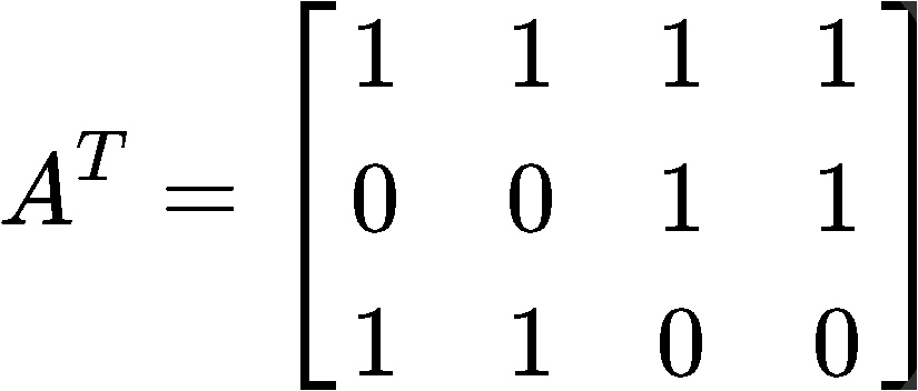
We start by finding the transpose $A^T$:


Next, we multiply the transpose to matrix $A$:


Now we multiply the transpose of matrix $A$ with the vector $b$:


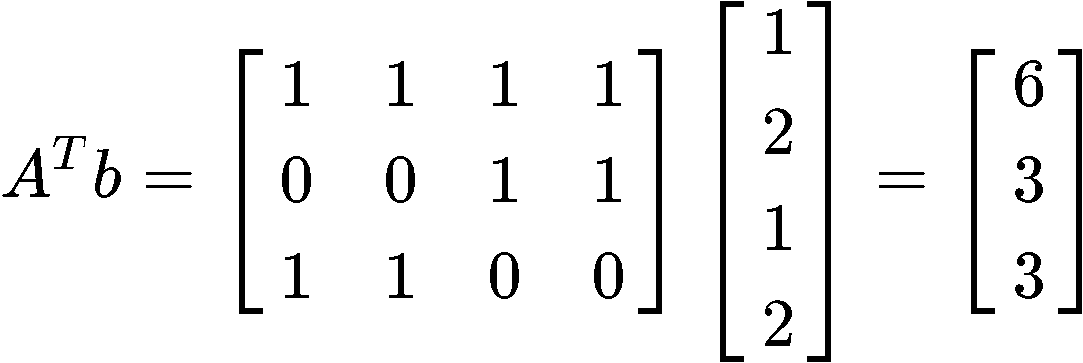
With the results found in equations 15 and 16, we can construct the matrix equation $A^TA\hat{x} =A^Tb$ as follows:


Transform the matrix equation above into an augmented matrix and row reduce it into its echelon form to find the components of vector $\hat{x}$:




And so, we can construct the least squares solution $\hat{x}$ with the components found:

Example 3

You are given that the least squares solution of $Ax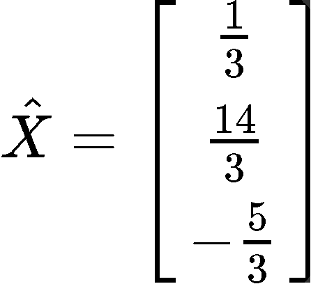=b$ is


Compute the least square error if $A$ and b are as follows:


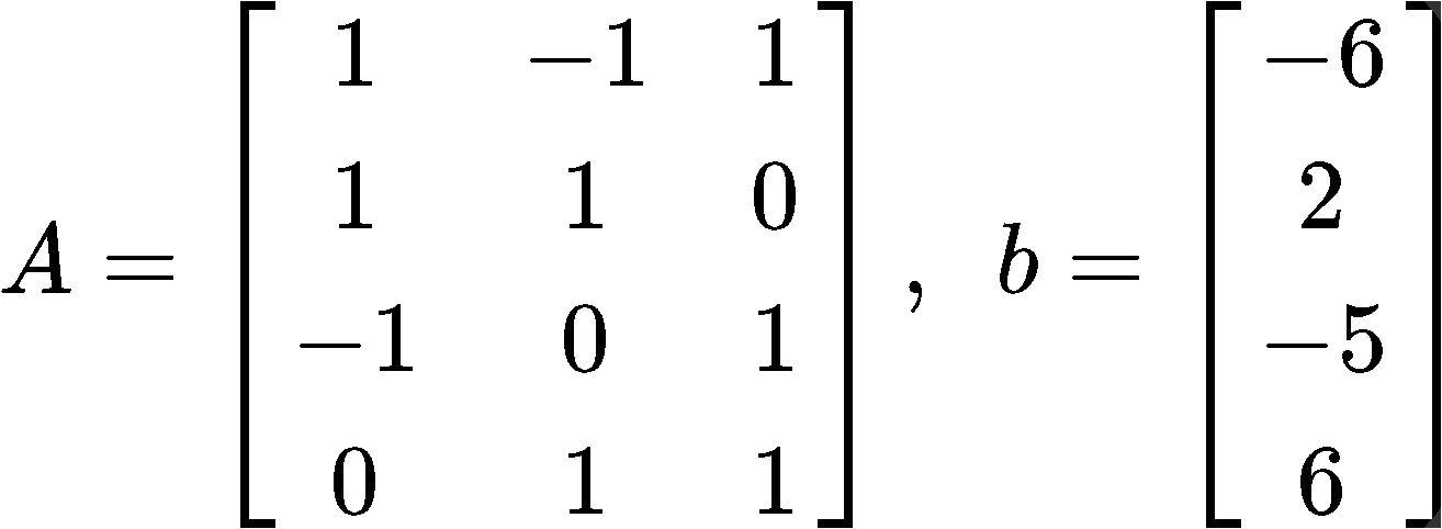
This problem is asking us to calculate the magnitude of the smallest possible error in $\hat{x}$. Such error is defined in equation 6, so now, we just have to follows the next simple steps to compute it:
Start by computing the multiplication $A\hat{x}$:


Having found the column vector from the multiplication above, we need to perform a subtraction of vectors by subtracting the vector found in equation 22 to vector b just as shown below:


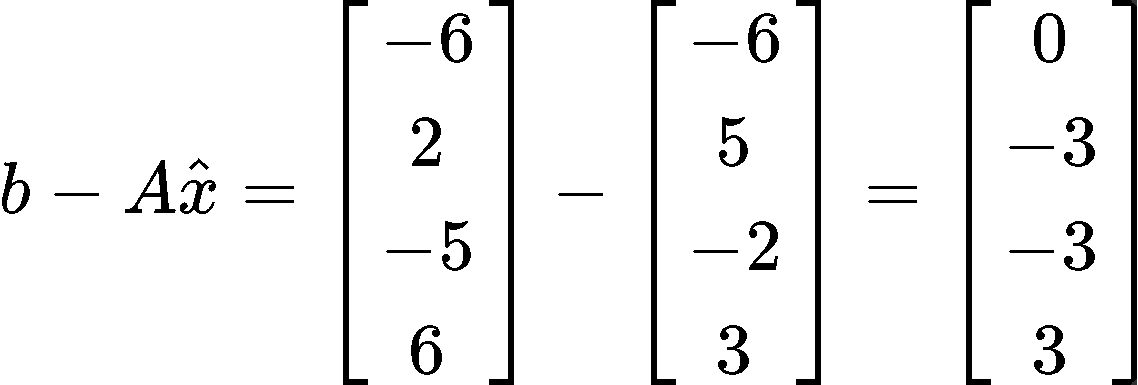
And now, you just need to find the length of the vector found in equation 23. Remember we do that by computing the square root of the addition of the components of the vectors squared:


And we are done, the least square error is equal to $\sqrt{27}$

Example 4

Find the orthogonal projections of $b$ onto the columns of $A$ and find a least-squares solution of 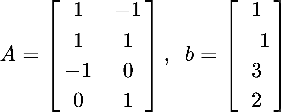$Ax = b$.


In order to find the orthogonal projections and the least squares solution for this problem we need to use and alternative approach, and so, for this case we start by computing the orthogonal projections of b onto the columns of $A$ using the formula found in equation 5, to the go ahead and solve for the least squares solution using equation 4.
For the orthogonal projections we have that:

$\large \hat{b} =$proj$_{Col(A)}b = \frac{b\cdot a_1}{a_1 \cdot a_1}a_1 \; +\; \frac{b\cdot a_2}{a_2 \cdot a_2}a_2$
Where $a_1$ and $a_2$ are the column vectors that compose the matrix $A$. Therefore, solving for $\hat{b}$ goes as follows:

$\large \hat{b} =$proj$_{Col(A)}b = \frac{(1)(1)+(-1)(1)+(3)(-1)+(2)(0)}{(1)(1)+(1)(1)+(-1)(-1)+(0)(0)}a_1 \; +\; \frac{(1)(-1)+(-1)(1)+(3)(0)+(2)(1)}{(-1)(-1)+(1)(1)+(0)(0)+(1)(1)}a_2 =-\frac{3}{3}a_1 \;+ \; 0a_2$

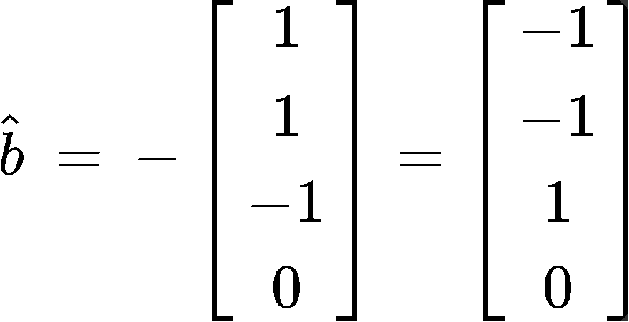
And so, we have found the orthogonal projections. Now for the least squares solution we use as reference equation 4 and take the matrix $A$ and vector $\hat{b}$ so we can form the matrix equation:


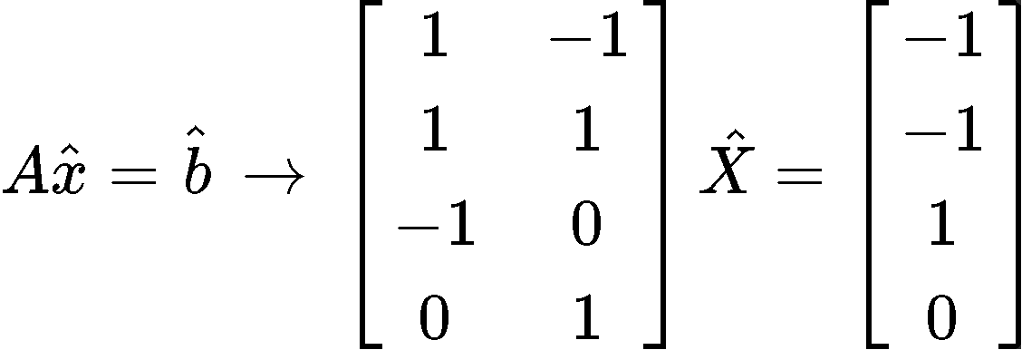
Where we can easily obtain the vector $\hat{x}$ since its components are $x_1 = -1 \;$and$\; x_2 = 0$, and so:



*** To finalize this lesson we would like to recommend you to take a look to this lesson on least squares that contains a thorough explanation of the topic plus some extra examples.
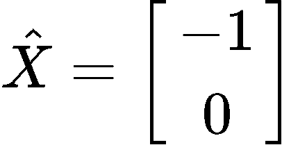
This is it for our lesson on least squares, we hope you enjoyed it, and see you in the next lesson, the final one for this course!