Row Reduction and echelon form
Through the last lesson we studied the method of solving a linear system with matrices using Gaussian elimination, and we talked about the two stages of this elimination technique and how some people have different names for them. Therefore, throughout this lesson we will continue talking about Gaussian elimination, but now usually calling it by its other name: row reduction method, and we will focus on the results from the mentioned two stages of it: the row echelon form and the reduced row echelon form of a matrix.
What is row echelon form
The matrix row echelon form (or simple matrix echelon form) is a simplified equivalent version of a matrix which has been reduced row by row. In order to understand completely what this type of matrix is and its characteristics we need to learn the next four basic concepts:
- A non-zero row is a row that has at least one entry that is not zero.
- The leading entry of a row is the left-most non-zero entry in a non-zero row.
- The pivot position is just the leading entries of the echelon form matrix.
- The pivot column is the column of the pivot position.
Therefore, any rectangular matrix is in echelon form if it has the next three properties:
If the rectangular matrix satisfies 2 more additional properties, then it is said this is a reduced echelon form matrix:
Essentially the difference between the definition of echelon form and the reduced echelon form is that the former has a value of 1 as all of its leading entries, and the leading entries columns have all zeros below and above.
How to row reduce
We have already practiced row reduction linear algebra with the exercises containing augmented matrices in the past lesson, this time we will focus on regular matrices (not augmented), they could be matrices with any magnitude combinations, and for that we usually call them rectangular matrices, but be remember that all of the operations shown in here can be applied to any type of matrix.
There is no specific set of steps about which of the three types of matrix row operations, or combinations of them, need to be used in order to perform row reduction to produce a row echelon matrix, or a reduced echelon matrix. But, we can think of a general algorithm with the steps for the process of reducing matrices into these echelon forms (which operations to use will be left for your intuition in each case, so practice is key!). And so, we have listed the algorithm below.
The steps for the row reduction algorithm:
*The next step is added to the algorithm when row reducing into the reduced echelon form (notice this next step is what would be called back substitution or the Gaussian Jordan elimination method).
Row echelon form vs. reduced row echelon form
We have mentioned before that reduced matrices into echelon form have only two differences to those in reduced echelon form. Let us take a look at the representation of these two types of matrices:
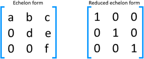
As you can see, each of them is a row reduced matrix with pivot points and a triangular configuration, but the matrix in echelon form can contain any values as its non-zero entries, while the one in reduced echelon form can only contain ones. Furthermore, the second difference comes from the fact that the matrix in reduced echelon form can only contain zeros either above of below its pivot points in each column.
Let us work through a few row echelon form examples so you can actively look for the differences between these two types of matrices.
Example 1
Label whether the matrix provided is in echelon form or reduced echelon form: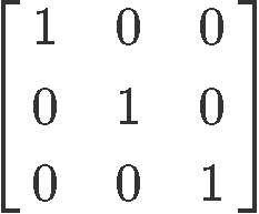
This matrix is in reduced echelon form because the leading entries for each row are all ones and they are the only non-zero entries on their corresponding columns. Notice the reduced echelon form of matrix in equation 2 is also what we call an identity matrix, from this we can obtain a new concept: If a reduced echelon form matrix is a square matrix without zero rows, this will be an identity matrix.
Example 2
Is this an echelon form or reduced echelon form matrix?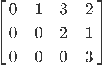
This matrix is in echelon form. We can fast identify this cannot be in reduced echelon form since a few of the leading entries differ from one. The characteristics that make this a matrix in echelon form is that the pivot in each row is to the right of the pivot in the row above it, besides, everything below each pivot is zeros.
Example 3
Label whether the matrix provided is in echelon form or reduced echelon form: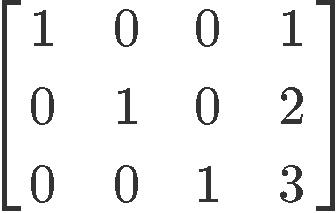
This matrix is in reduced echelon form due to the next two reasons:
All of its pivots are ones and everything above or below the pivots are zeros.
Example 4
Is the next matrix in echelon form or reduced echelon form?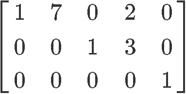
This particular matrix is in reduced echelon form. Notice that this can be tricky to identify since you have many columns with different values which are not either one or zero. The reason why this is an example of a matrix in reduced echelon form is that all of the leading coefficients are ones, and in the corresponding columns of the leadings coefficients you can only find zeros on top or below them.
So it doesnt matter that the second and fourth columns have coefficients different to one or zero, as long as the coefficients above or below the pivots are zero, and the pivots themselves are ones (and of course remember that each pivot must be to the right of the pivot in the row above it) you have a matrix in reduced echelon form.
Reducing a matrix to row echelon form
The process to reduce to echelon form or reduced echelon form is essentially the same as you can observe from the row reduction algorithm above. The main difference comes from the fact that obtaining the reduced echelon form tends to take longer time since you need to make sure all the leading coefficients (or pivots) are ones and all the elements either above or below them in their corresponding columns must be zeros.
Now we will work on finding the general solutions to augmented matrices, this with the purpose of solving systems of differential equations.
From the lesson on representing a linear system as a matrix we learnt that in order to find the general solution to an augmented matrix we need to find the reduced row echelon form of the matrices representing such linear systems, therefore, for the next examples we will be row reducing the given matrices into their respective row reduced echelon form to start practicing this process. We will later find the general solutions of the matrices in the next set of examples.
Example 5
Row reduce the next matrix to reduced echelon form. Circle the pivot positions in the final and original matrices, and list the pivot columns from the original matrix.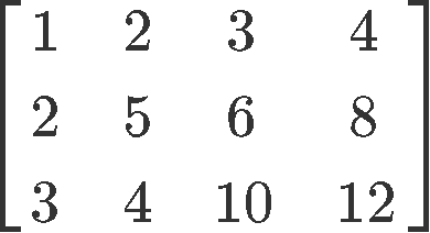
Following the row reduction matrix method:


Therefore the reduced echelon form of the matrix in equation 6 is:
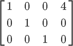
Circling the pivot positions in the final and original matrices, and marking the pivot columns from the original matrix:
Example 6
Row reduce the next matrix to reduced echelon form. Circle the pivot positions in the final and original matrices, and list the pivot columns from the original matrix.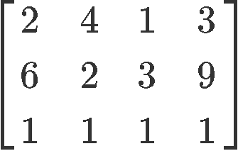
Row reduce matrix in equation 10:


Therefore the reduced echelon form of the matrix in equation 10 is:
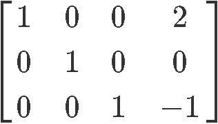
Circling the pivot positions in the final and original matrices, and marking the pivot columns from the original matrix:
Next, for the following examples we will be computing their general solutions, for which we need to perform matrix reduction to reduced echelon form first, and then obtain the general solution for the variables in the system of equations from which the augmented matrices come from. Notice these problems are very similar to those seen in our last lesson.
Example 7
Find the general solution of the following matrix:
Computing the Gaussian elimination to produce the reduced echelon form matrix and write down the system of equations corresponding to this case:


Looking at the resulting system of equations we can obtain the general solution to the matrix by noting the solution value for each of the variables in it:
Looking at the columns on the left hand side of the matrix after the reduction process we can now define two types of variables that an echelon and reduced echelon form matrix can have. In equation 15 we can see how the first and second column (corresponding to variables and ) contain a pivot, while the third column (corresponding to variable ) does not. This means that variables and are basic variables, while is a free variable. Free variables are those which can take any constant value and will not change the proportionality of the system of equations or the augmented matrix equation. But there is a catch, if we have a free variable which can take ANY constant value as its own, this means this particular system can have an infinitesimally amount of possible solutions!
Example 8
Find the general solution of the following matrix: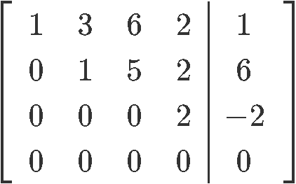
This particular matrix is already in echelon form, but since we are looking for the general solution of the matrix we need to obtain its reduced echelon form first. Thus, let us row reduce it into its reduced echelon form:


As you can see from the matrix in reduced echelon form , , are basic variables since all of them have a pivot on the matrix. The free variable of this matrix is since there is no pivot for it, and we can see this by solving the resulting system of linear equations in order to find the final general solution:
As final exercises we will look into an application of row reduction and echelon forms: finding out if a system of linear equations can have infinite solutions or if it just cant be solved (no solutions).
Example 9
Choose values of and where the system has infinitely many solutions, and no solutions:
Remember that in order to have infinitely many solutions it means you need to have a free variable in the system. Thus, what we will be looking for in here is to find a free variable. Why is it that we need a free variable? Because a free variable is that which can have ANY value and so, by changing the value of that particular free variable to ANY number, then you can have an infinite amount of possible solutions for the whole system.
For this matrix case to have a free variable means that the second row should be all zeros, thus we row reduce the matrix in order to obtain an expression for the second row that would allow us to convert it to all zeros by inputting certain values to and :

And so, in order to make the second row to be all zeros, the values that and must be: and \, b= {8.
Now, the other way around is when you have no possibility to obtain a solution for the system you are given. This happens when you have an inconsistent row in the augmented matrix you are working on (something saying zero is equal to any other constant for example), sometimes this can leave you with less equations than the unknowns you have to solve for and so, there is no way to obtain the solutions to all of the variables involved.
Then, for the reduced augmented matrix in equation 21 to have a second row which is inconsistent a and b must get the values of: and ≠ .
Example 10
Choose values of and where the system has infinitely many solutions, and no solutions:Then, we need to obtain the corresponding augmented matrix and row reduce it to find an expression on the second row where we can find the values for a zero row, or an inconsistent row.

And so, for the case of infinitely many solutions the values of a and b must be: and
Then for the case of no solutions: and ≠ .
To finish up with this lesson, we would like to recommend you to visit these two lessons on row reduction and echelon forms which contain not only different forms of a row reduction example, but extensive explanations on the topic.
We hope you have enjoyed this lesson, see you in the next one!
A non-zero row is a row that has at least one entry that is not zero.
The leading entry of a row is the leftmost non-zero entry in a non-zero row.
A rectangular matrix is in echelon form if it has the three properties:
- All non-zero rows are above any rows of all zeros.
- Each leading entry of a row is in a column to right of the leading entry of the row above it.
- All entries in a column below a leading entry are zeros.
If the rectangular matrix satisfies 2 more additional properties, then it is in reduced echelon form:
- The leading entry in each non-zero row is 1.
- Each leading 1 is the only non-zero entry in its column.
Essentially the difference between the two forms is that the reduced echelon form has 1 as a leading entry, and the column of the leading entry has 0's below and above.
The pivot position is just the leading entries of the echelon form matrix.
The pivot column is the column of the pivot position.
Here are the steps for the row reduction algorithm:
- Look for the leftmost non-zero column. This is our pivot column.
- Find a non-zero entry in the pivot column. This is our pivot position. It should be at the very top of the pivot column.
- Use matrix row operations to make all the entries below the pivot 0.
- Ignore the row with the pivot. Repeat Step 1-3 again and again until you can't anymore.
- Find your rightmost pivot. Make it 1. Then make all the entries above it 0.


