Linear Combinations and Vector Equations in R^n Explained

Dive into the world of linear combinations and vector equations in R^n. Understand key concepts, learn problem-solving techniques, and apply your knowledge to real-world scenarios in physics, engineering, and data science.

Linear combination and vector equations Rⁿ

Throughout the past lessons we have studied the notation of matrices, worked with systems of linear equations and learned how to represent them and solve them by either graphing or matrix row reduction. The time has come for us to learn about the usage of such notations and techniques when working with linear combinations and vectors, and for that reason, let us have a little introduction about vector notation in matrix form and the plane dimensions of such vectors before we enter into the main topic of today.
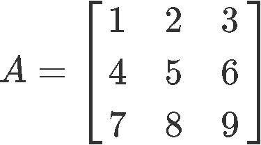
Recall a matrix is an array of numbers put in a rectangular bracket which dimensions are defined by how many rows and columns it has. So, a simple 3x3 matrix looks like this:


A matrix with one column is called a column vector and it can be used in different algebraic operations along with other column vectors.


The column vector is said to be in coordinate space $R^{2}$ since it has two rows of real numbers, this means the vector has two dimensions and its graphic representation would lie on a two-dimensional plane. We can also have a vector in $R^{3}$ which could be a three-dimensional vector such as the one below:


You can actually have a column vector with as many rows as you want, and so, we say a vector is in the coordinate or vector space $R^{n}$ where n will define how many rows are contained on it. We can summarize that a vector in $R^{n}$ would have n entries in one column, such as:


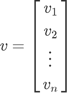
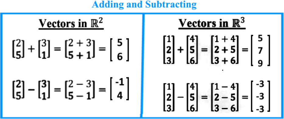
The amount of rows in a column vector is very important to denote the type of vectors you can operate with one another. Plainly said, column vectors can be added or subtracted with other column vectors only as long as they have the same amount of rows.


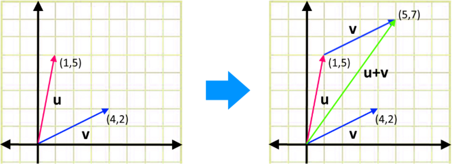
To add or subtract vectors take us to an important concept called the parallelogram rule of addition. The parallelogram rule of addition is used when working on the graphic representation of vectors, and it states that when adding two vectors we can represent them as the adjacent sides of a parallelogram drawn from the origin, which means that you are to move a vector parallely from its original position to have its tail start from the arrowhead of the other, and the resultant vector from such addition (or subtraction) would have the magnitude and direction resulting from this new vectors tail being in the origin (the starting point) and running until the arrowhead of the outermost vector. The graphic representation of the addition of two vectors is shown below:


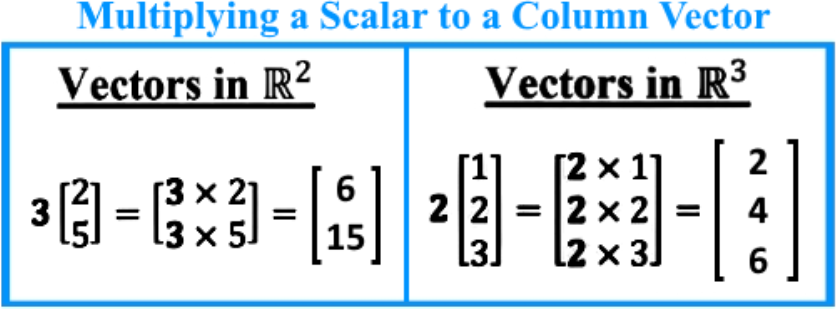
We can also multiply a column vector by a scalar:


And so, to operate (add, subtract, or multiply a scalar) on vectors, here are the following properties of $R^{n}$, where $u$, $v$, $w$ are vectors and $c$, $d$ are scalars:

What is a linear combination

Given vectors $v_{1}$, ...,$v_{p}$ in $R^{n}$ with scalars $c_{1}$, ... ,$c_{p}$, the vector equation $x$ is defined as:

$x=v_{1}c_{1} + v_{2}c_{2} + ... + v_{p} c_{p}$
Where x is a linear combination of vectors $v_{1}$, ...,$v_{p}$ with scalars $c_{1}$, ... ,$c_{p}$.
The linear combinations of $v_{1}$, ...,$v_{p}$ is the same as saying this is a linear combination span: Span{$v_{1}$, ...,$v_{p}$}

There is something very important to note in this kind of notation before we continue on the section teaching about vector equations. For the linear combination definition we just saw above, the range of $v_{1}$, ...,$v_{p}$ refers to the range of column vectors and the scalars are by definition magnitude values because we usually refer to this as a value of one (this is always the case for linear combinations which would result in linear systems of equations). The reason to use a value of one for the scalars comes from the fact that we will be converting such linear combinations into vector equations, which later can be transformed into augmented matrices which by now, we know can be re-written as a system of equations.

Therefore, by the time such transformations (or transcriptions) of such linear combinations to a system of linear equations finally occur, we will see how such scalars hereby named $c_{1}$, ... ,$c_{p}$ actually represent the variables in the equation which provide the dimensions for the graphic representation of such systems of linear combinations.

At the moment this all may seem rather confusing, so let us get into the next section where we will explain step by step the method of going from a linear combination notation such as the one shown in the definition in equation 8 to the algebraic notation representing a system of linear equations, passing through vector equations and augmented matrices in the process.

What is a vector equation

Equation 8 has so far been called the definition of the linear combination, in truth, this is also a vector equation, so it is now time for us to take it as such and expand it. How to do it? Actually we have already hinted in the past section it is all about linear systems of equations, so now, let us represent a system of linear equations as the vector equation from the definition in equation 8:


Notice what has been done here. We took a system of linear equations which can be found in the left-most side above and wrote them as a vector equation notation by separating the terms with distinct variables and finally (in the right-most part), provide a vector equation in which you can clearly see the values corresponding to the two ranges of terms defined by $v_{1}$, ...,$v_{p}$ and $c_{1}$, ... ,$c_{p}$. Remember that $v_{1}$, ...,$v_{p}$ refers to column vectors, and $c_{1}$, ... ,$c_{p}$ as scalars, so:


The vector equation resulting from the linear system of equations is:


Thus we can say a vector equation such as the one shown in equation 11 is a linear combination if its left hand side is equal to its right hand side, which can only happen when the scalars x1,x2,x3 are all equal to one.

To elaborate on this explanation and make the relationship between a linear system of equations and a linear combination clearer, let us remember what we had mentioned before: the array $v_{1}$, ... ,$v_{p}$ refers to the column vectors, while $c_{1}$, ... ,$c_{p}$ end up referring to the variables of the system of equations, in this case $x_{1}, x_{2}, x_{3}$. This is the confusion we were trying to clear out in the last section, why do we call $x_{1}, x_{2}, x_{3}$ scalars if we know that when transcribing them from a system of equations, they happen to be the variables? Because they have a value of 1. Since we are ONLY talking about systems of linear equations, by definition, these variables would have a magnitude of one since this is the only value that allows the left hand side and right hand side of equation 11 to be equal.
In other words, the system of linear equations in the left-most side of equation 9 and equation 10 could be very well written as:


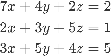
How do we know that? Well it so happens that if you have a vector equation, similar to the one found in equation 11, we can write it as an augmented matrix. Take the example below:


Which, as we know from our lesson on representing a linear system as a matrix, an augmented matrix notation follows the next rules:


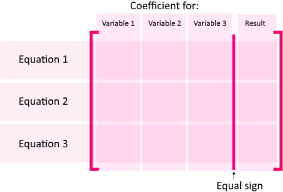
Which means that variable 1, variable 2 and variable 3 are the same as $x_{1}, x_{2}, x_{3}$ or just $x$, $y$ and $z$, it really does not matter which name you give to them! For this lesson we will be looking into the linear combination of normal random variables.


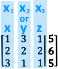
Once we have the augmented matrix we know how to solve it! Remember from our lessons on solving a linear system with matrices using gaussian elimination and rrow reduction and echelon formswe learned the technique to use the three types of matrix row operations in order to solve a system of linear equations. So, if you have any doubts on how row reduce the matrix shown above in equation 14, we recommend you to go back and do a little review of the lessons suggested here. Also, do not forget to check out the videos accompanying this lesson, since all of our operations have been shown in there.

Linear combination method examples

As the title of this lesson describes, it is time now we work on exercises which represent linear combination examples. Notice we will go advancing step by step throughout the exercises, from how to write vector equations to how to find a vector linear combination, which can be found in the last problems which we will solve by linear combination.

Example 1

Consider the two vectors shown below and then compute the operations in parts a), b) and c):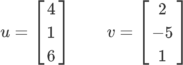


Compute

Example 2

Using the next system of equations, write it as a vector equation: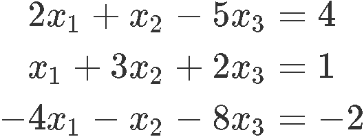


In order to write the linear system as a vector equation, we start by separating all of the terms containing the same variable as columns, and then rewrite them as such:



As you can see in equation 20, the right-most equation is the one consisting of the vector equation form in which the variables $x_{1}$, $x_{2}$ and $x_{3}$ are multiplying a column vector comprised of the coefficients found in the system for each variable.

Example 3

Write the given vector equation as a system of equations:


We just easily distribute the coefficients to each of the variables:



***
For the next example, we will be using the linear combination method in order to find a vector parametric equation with explicit values, which will allow us to confirm if the given elements are linear combination vectors.

Example 4

For $b$ to be a linear combination with the given column vectors $a_{1}$ and $a_{2}$ are added, it means that the vector equation you can construct with these terms will have equal values on its left hand side and on its right hand side. Therefore, we start by writing the vector equation from the given column vectors and convert it into the augmented matrix:


What we need to do here is to find the values of $x_{1}$ and $x_{2}$ by computing the reduced echelon form of the augmented matrix using row reduction. If we can obtain a particular value for each, then it means b is a linear combination of $a_{1}$, $a_{2}$, and so, we row reduce to solve for the unknown variables:



Since we were able to solve for the variables $x_{1}$ and $x_{2}$ without and issue, then we can see that b will be a linear combination for $a_{1}$ and $a_{1}$ when:

$x_{1}= \frac{34}{4} = 8.5$ and $x_{2} = 8$



Again, we write down the vector equation, transform it into the augmented matrix and then row reduce it to find the values of the unknown variables:







And as you can see, since we could find the value of all the variables, then b is a nontrivial linear combination of $a_{1}$ and $a_{1}$.

***
We finalize the lesson here after having done linear combination of matrices examples. Before we pass into the next lesson, we recommend you to take a look into these lessons on linear combinations and vector equations, where you will find even more examples and also, some graphic representations of the equations and systems we have seen today.