Equilibrium Solutions
Equilibrium point definition
When talking about physical systems we use the term equilibrium to describe a system that doesn't change, that is in balance. We translate this same concept to mathematics when talking about the behavior of functions as you graph them and how you can observe its dependent value to stay balanced through different values of the independent variable.
So what does equilibrium mean in this case? From the point of view of slopes and differential equations, equilibrium refers to a value of zero in the inclination of a graphed function. This means that for an equilibrium point in this function, the function's value is a constant. This in turn concludes that for a differential equation with a solution function, this solution to the differential equation is equal to a constant value making its derivative (slope of the tangent line) equal to zero. Therefore, a constant solution to a differential equation when this differential equation is equal to zero, is called an equilibrium solution or just the "equilibrium point" (as mentioned before), where the graphed line of the function is horizontal.
Remember that when graphing a function, depending on its inclination direction, you can easily identify the sign of the value of its slope at different points. For simple reference take a look at the next figure:
So when a graphed function shows an "uphill" inclination its slope is positive, meaning the derivative of the function with respect to the independent variable will result in a positive value as well. In the same manner, when the function's inclination is "downhill" it means the slope of the function is negative, and the derivative of the function will produce a negative result.
For this lesson we will be paying attention to the third case, where the function is running horizontally and its slope is zero, determining the solution equilibrium definition: the value of the function's derivative related to the independent variable is zero and so, the function is in equilibrium at those particular points.
For further review on slope fields and their characteristics, make sure to revisit that particular lesson in StudyPug. We recommend that if you are not familiar with the terms used so far in this article, you go ahead and study that lesson first and then come back later to continue with your equilibrium points studies.
How to find equilibrium solutions
When having a differential equation we say the solution is an equilibrium solution if the derivative of it with respect to the independent value is equal to zero. This means the slope of the tangent line of the function is horizontal, balanced and so it has a zero value of inclination.
For this reason, in order to obtain the values of y which represent the equilibrium solutions or equilibrium points, we set the derivative of y with respect to the independent variable equal to zero and solve for y. We will be working a few examples of this, but before we get into it, let us just say that the process in itself requires usually simple algebra such as factorization of polynomials, and in the case of quadratic equations we can simple use the quadratic formula to solve for them.
Having found the values of y that represent equilibrium points, we are left to determine their stability. We do this by finding the slopes of solutions to the function at different values of y.
In other words, the differential equation can have multiple solutions depending on different values of y, is just that we are not truly interested on them because they are not all equilibrium points. But after having found these primordial ones to us, we check on the nearby surrounding solutions and calculate their slopes to pay attention to their signs. A positive or negative sign in a slope, gives us the general inclination orientation of it, and therefore it will let us know if the function to which they belong is either coming towards our equilibrium solution, or getting away from it as the independent variable increases.
These characteristics will tell us if our equilibrium solutions are stable or unstable. A Stable Equilibrium Solution is that to which all solutions "near" converge on it. An Unstable Equilibrium Solution is that which all solutions "near" to diverge from it
Find the equilibrium solutions of the autonomous differential equation
An autonomous differential equation is that which is defined as the equality of a derivative in which the independent variable (usually named either x or t) only appears as the base for the derivative and nowhere else in the equality. Simply said, an autonomous differential equation contains a derivative in one side of the equal sign and in the other side, the function found is only in terms of the dependent variable and constant coefficients. This can be easily seen in the mathematical expression for it:

Notice that in these two general representations for autonomous equations, the independent variables x and t (for each case) are only found deriving the variable y, but they do not appear in the right hand side of the equations.
A great example of an autonomous equation is the logistic differential equation for population growth since you can see the way how population changes through history as time progresses. Therefore, this equation is the derivative of P with respect to t (or the rate of change of the population, denoted by P, with respect to time, denoted by t). The logistic growth model equation looks as follows:

Where K and M are constants.
As you can see from this growth equation, we can simply call it a function of P since the right hand side is defined just in terms of P and that is what makes it autonomous.
It can be easily understood why a formula describing the way population changes through time is actually independent of it. Time passes by does not matter what, it is a dimension we live in so we have to measure the change as it passes by and us with it, but it does not truly make a difference on how a population of a species grows or changes, it has no influence on it. Several other factors can have an effect on how the population of a species (any species of a living organism) behaves: environmental factors, the increase of predators or decrease of them, the way they migrate to different regions and the conditions they find on their way, etc. All of those are factors related to the population alone and how the organisms themselves make decisions and behave due their capacities. And so, the growth of a population depends on the population alone and the equation describing this independency ends up being an autonomous differential equations for that reason.
Note:
The growth formula seen above is a simplistic analogy of the use of an autonomous differential equation. Although in theory is correct, this is based on a small reference frame without taking into account the vastness of geological time and the development and influence this has into an species progress. So, although for our math purposes of today is completely correct, geologists and astronomers (mostly cosmologists interested in relativity) may argue that we are leaving many variables out of our equation and that time can actually be wrapped and bent and not just let it be, this of course would take entire courses to be described and the influences of such distortions are so particular that are not truly practical for our topic of today. So let us take it in this simplistic form for now, but if you are ever interested on these topics do not hesitate to contact StudyPug and ask for them!
For other physical applications of the logistic model (this can be apply to many other things besides population growth!) we suggest you to visit this article on equilibrium to see a general form of the model. Also, for further reading on equilibrium points take a look at these notes.
Knowing this, we are about to find the equilibrium solutions of an autonomous differential equation in our first example, as always we will make the effort to list the steps followed through this process so you can use them when working in different practice problems.
Example 1:
Find the equilibrium solutions of the differential equation shown below and classify each equation solution as stable or unstable:

-
In order for us to find the equilibrium solutions of the ordinary differential equations we need to find the values of y when the slope of the equation is in equilibrium and this is when the derivative of y with respect of t is zero. Therefore, we set the equation on top equal to zero and find the values of y:

Equation for example 1(a): Finding the equilibrium solutions for the ordinary differential equation Therefore the equilibrium solutions to the ordinary differential equation for this problem are y=4 and y=-1. Now we need to find out if they are stable or unstable solutions and for that we will solve the ordinary differential equation for different values of y and see if the slope of y for that value is positive or negative.
-
Note:
Remember that for values of y above a point of equilibrium if the slope is positive it means the function is diverging, if the slope is negative then the function is converging. In the other case, when looking at values of y smaller than the point of equilibrium, a positive slope means a converging function, and a negative slope means it is diverging.
These characteristics are shown in the graphs below where we have selected a random equilibrium point of y=3 just for practical purposes:
-
Let us continue with our example and find the values of the slope (differential equation) for values of y higher than 4. This can be done by substituting the wanted value of y on the first equation for example 1:
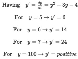
Equation for example 1(b): Finding the slope sign for y values higher than 4 -
Now repeating the same process for values of y ranging between -1 and 4:
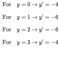
Equation for example 1(c): Finding the slope sign for y values between -1 and 4 -
Lastly we repeat the process again but now for values lower than -1:
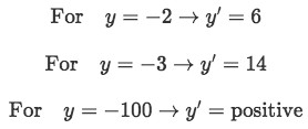
Equation for example 1(c): Finding the slope sign for y values between -1 and 4 -
We graph this outcome to see how these slope values relate to the equilibrium solutions to differential equations:
As you can easily observe from the graph at y=4 we have an unstable equilibrium solution since surrounding solutions nearby move away (diverge) from the equilibrium point as t increases. On the other hand, for y=-1 we find that we have a stable equilibrium solution, since the nearby surrounding solutions move towards the equilibrium point as t progresses.
Before continuing onto our second example, let us list, as always the clear steps for equilibrium points differential equations problems:
-
Set the differential equation equal to zero and find the equilibrium solutions.
- Remember in here we need to define the derivative of y (the dependent variable) with respect to t or x (whichever our independent variable in the problem is) equal to zero, since this derivative represents the slope of the tangent line to our graphed function y. And so, by setting the derivative equal to zero we solve for y with the certainty that any result y yields will be an equilibrium result, because those are the values of y that yield a y'=0.
- In order to find the solutions to y we use simple algebra methods such as factoring polynomials, etc
-
Having the values of y which represent equilibrium points we can now plug different values of y into our differential equation to find out the slopes at different locations in the graph.
- The values of the slopes (more importantly, their signs) give the orientation of the solutions nearby our equilibrium points and thus they can tell us if such solutions above or below our equilibrium point in question are either converging or diverging.
- If nearby solutions to the equilibrium point are all converging towards it, then we have a stable equilibrium point, if the nearby solutions are all diverging then we have an unstable equilibrium point.
- There could be a case in which solutions above the equilibrium point are diverging while the solutions below are converging (or vice-versa), for such case we say we have a semi-stable equilibrium point, since is neither converging not diverging.
- (OPTIONAL) We can also draw the graphic representation of our equilibrium points in a cartesian coordinate system, and then plug the directions of the slopes of nearby solutions to easily see if they either converge or diverge towards our equilibrium solution. We recommend to follow through this step if you prefer visual aids while studying, this will help you identify the stability of the equilibrium solution in a faster and easier manner. Examples of such graphs can be found in figures 2, 3 and 4.
Example 2:
Now let us work on our final example for equilibrium solutions and stability differential equations. For the following autonomous differential equation define equilibrium points and identify if these equilibrium equations each represent either a stable solution or an unstable solution.

-
Step 1:
Set the differential equation equal to zero and find the equilibrium solutions.

Equation for example 2(a): Finding the equilibrium solutions for the ordinary differential equation In this case, finding the equilibrium point values were very easy to obtain since the equation had the binomials already associated in a form that is easy to see the equalities once you set the equation equal to zero.
-
Step 2:
Having the values of y which represent equilibrium points we can now plug different values of y into our differential equation to find out the slopes at different locations in the graph, let us do this by parts.
For values of y higher than 1:
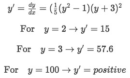
Equation for example 2(b): Finding the slope sign for y values higher than 1 For values between 1 and -1:
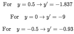 x
x
Equation for example 2(c): Finding the slope sign for y values between 1 and -1 For values between -1 and -3:
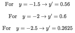
Equation for example 2(d): Finding the slope sign for y values between -1 and -3 For values lower than -3:
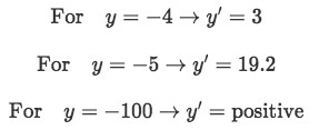
Equation for example 2(e): Finding the slope sign for y values lower than -3
Just by looking at the slope values gotten in the past calculations, we can conclude that the equilibrium point found at y=1 has all the nearby solutions diverging away from it, and so this point is unstable. Then for the equilibrium point and y=-1 we have all of the surrounding solutions converging towards it, and so, we have a stable equilibrium solution.
But now let us pay attention to the equilibrium point at y=-3, the solutions above this point are going away from it (diverging) as x increases, while the solutions below this point are getting towards it (converging) as x increases, so this equilibrium point is neither stable or unstable. We call these cases a semi-stable equilibrium point since it has solutions converging towards it from one side, but diverging from it from the other.
To have a visual representation of this we have included the equilibrium points and the slopes of the surrounding solutions for them graphed in the next figure:
Notice that for this article we have included the graph of the general direction for the slopes of the surrounding solutions to the equilibrium points, that means that we have only graphed if they are getting away from (diverging) or coming towards to (converging) the equilibrium solutions for each problem, but these orientations are not exact (their inclination has not been graphed accurately, they are just there for general orientation purposes).
For a thorough explanation on how to graph differential equations for these problems, do not forget to watch the videos on top of this lesson completely. We also recommend to take a look at the examples found on these differential equations notes.
Note the Logistic Equation:
With and being constants. This is a function of .
This is an example of an Autonomous Differential Equation.
An Autonomous Differential Equation is a differential equation that is of the form:
If we can find a solution such that for some , then this will be an Equilibrium
Solution.
A Stable Equilibrium Solution is an equilibrium solution that all solutions "near" to this equilibrium solution converge on it.
An Unstable Equilibrium Solution is an equilibrium solution that all solutions "near" to this equilibrium solution diverge from it


