Linear Approximation
Let's say that one day you forgot a calculator and you really want to find how what the square root of 2 is. How would we find out without a calculator? We can use linear approximation!
Linearization of a function
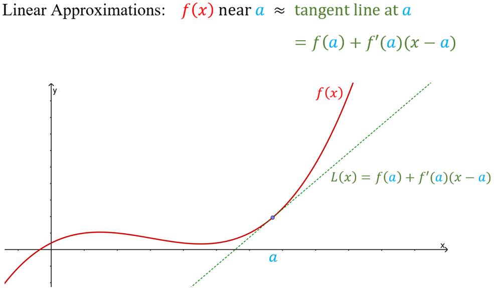
The linearization of a function is just about finding the tangent line of the function at a specific point in a different way. The linearization formula is:

where L(x) is the equation of the tangent line at point a.
How is this useful to us? Well, we can actually use this equation to approximate values of the function near point a. Take a look at this graph.
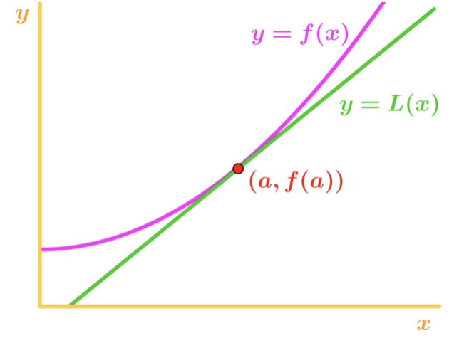
Notice that for x values near point a, we see that the function and the tangent line is relatively close to each other. Because of this, we are able to write that the function is approximately equal to the tangent line near point a. In other words,

where is the approximately symbol. This equation is known as the linear approximation formula. It is linear in a sense that the tangent is a straight line and we are using it to approximate the function. Using this approximation, we are able to approximate values that cannot be done by hand. For example, the square root of 2 or the natural log of 5 can all be approximated! One important thing to note is that this approximation only works for x values near point a. If you have a x value far from point a, then the approximation becomes really inaccurate.
Now don't we take a look at a few examples of finding the linearization of a function and then look at how to use linear approximation!
Find the linearization of L(x) of the function at a
Question 1: Consider the function

Let's say that we want to find the linearization of the function at point a=4.
To find the linearization L(x), recall that

Notice that in order to calculate L(x), we need f(a), f'(a) and a. Afterwards, were going to have to plug in everything in the formula to find L(x). Hence, I created these steps:
- Step 1: Find a
- Step 2: Find f(a)
- Step 3: Find f'(a).
- Step 4: Plug all three into the formula to find L(x)
Let's follow these steps!
Step 1: Luckily a = 4 is given to us in the question, so we don't have to look for it.- Step 2:
Notice that

Equation 1: Linearization question pt. 3 - Step 3:
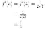
Know that the derivative of square roots is

Equation 1: Linearization question pt. 4 And so plugging in x=a gives us:
Equation 1: Linearization question pt. 5 - Step 4:
Since we know a, f(a), and f'(a), we can now plug it into L(x) to find the linearization of f(x).
Hence,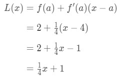
Equation 1: Linearization question pt. 6 So L(x)=x+1 is the linearization of this function at point x=4. In addition, it is also the tangent line of the function at point x=4.
How to do linear approximation
Remember earlier we said that we could use the equation of the tangent line to approximate values of the function near a? Let's try this with the linearization we found earlier. Recall that

for points near x=4. We can change this into a linear approximation for f(x) by saying that:

Now, let's say I want to approximate f(4.04). If you were to plug this into the original function, then you would get . This would be really hard to compute without a calculator. However, using linear approximation, we can say that
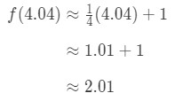
We just approximated the f(4.04) without a calculator! Now let's actually see how close we were to the exact value of f(4.04). Notice that f(4.04) = = 2.00997512422... So we are really close! We were only off when we've got to the second decimal place!
Now so far, these questions gave us a function and a point to work with. What if none of these were given at all? What if the question only tells us to estimate a number?
Use Linear approximation to estimate a number
Suppose we want to estimate . How would we do it? We would need to use the linear approximation

but we don't even have a function and a point to work with. This means we have to make them ourselves. This leads us to do the following steps:
- Step 1: create a function
- Step 2: create point a
- Step 3: Find f(a) and f'(a)
- Step 4: Plug everything into the linear approximation formula
Let's follow the steps!
Question 2: Estimate
- Step 1: Let's come up with a function. Note that we are estimating
We need to somehow make a relationship between f(x) and . We can't say that f(x) = because the function won't be dependent on x. So why don't we do this? Let

Equation 3: Estimate with linear approx. pt.2 If we do that, then we are basically saying
Equation 3: Estimate with linear approx. pt.3 We can now obviously tell what the function should be. Let
Equation 3: Estimate with linear approx. pt.4 So we have a function, but now we need a point a to work with.
Equation 3: Estimate with linear approx. pt.5 - Step 2:
The key to finding the right value a is by considering two things:
1) Make sure that the value a is close to x
2) Make sure f(a) is a nice number.
Would a = 8 be sufficient enough? Well, 8 is pretty close to 10 so it is not bad. However,

Equation 3: Estimate with linear approx. pt.6 Notice that is not a very nice number. In fact, you get a bunch of decimal numbers. So we have to try something else.
Would a = 9 be sufficient enough? Again, 9 is pretty close to 10 so it is okay. Also,

Equation 3: Estimate with linear approx. pt.7 f(a) is actually a nice whole number here, so this actually works! So picking a=9 is sufficient enough.
- Step 3:
Note that from earlier:

Equation 3: Estimate with linear approx. pt.8 Calculating f'(x) we have again:

Equation 3: Estimate with linear approx. pt.9 So
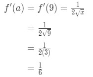
Equation 3: Estimate with linear approx. pt.10 - Step 4:
Going back to the linear approximation formula we have:

Equation 3: Estimate with linear approx. pt.11 Plugging a, f(a), f'(a), f(x), and x in our formula you will see that:
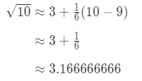
Equation 3: Estimate with linear approx. pt.12 Hence, we just approximated the number!
If you want more practice problems about linear approximation, then I recommend you look at this link here.
http://tutorial.math.lamar.edu/Classes/CalcI/LinearApproximations.aspx
Overestimate and Underestimate
We know that linear approximation is just an estimation of the function's value at a specified point. However, how do we know that if our estimation is an overestimate or an underestimate? We calculate the second derivative and look at the concavity.
Concave up vs Concave down
If the second derivative of the function is greater than 0 for values near a, then the function is concave up. This means that our approximation will be an underestimate. In other words,

Why? Let's take a look at this graph.
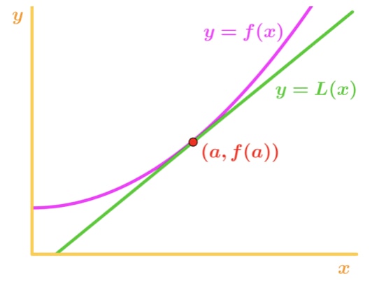
Notice that f(x) is concave upward and the tangent line is right under f(x). Let's say were to use the tangent line to approximate f(x). Then the y values of the tangent line are always going to be less than the actual value of f(x). Hence, we have an underestimate
Now if the second derivative of the function is less than 0 for values near a, then the function is concave down. This means that our approximation will be an overestimate. In other words,

Again, why? Let's take a look at another graph.
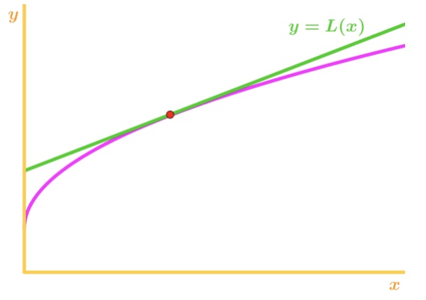
Notice that f(x) is concave downward and the tangent line is right above f(x). Again, let's say that we are going to use the tangent line to approximate f(x). Then the y values of the tangent line are always going to be greater than the actual value of f(x). Hence, we have an overestimate.
So if you ever need to see if your value is an underestimation or an overestimation, make sure you follow these steps:
- Step 1: Find the second derivative
- Step 2: look at the concavity of the function near point a
- Step 3: Confirm that it is an underestimate/overestimate
Let's take a look at an example:
Question 3: Let f(x) = and a = 4. If we linear approximate f(4.04), would it be an overestimate or an underestimate?
- Step 1: See that
So the second derivative is

Equation 4: Overestimate question pt.1 
Equation 4: Overestimate question pt.2 - Step 2:
Notice that a=4, so we want to look at positive values of x near 4. Now look at the second derivative. When x is positive, we see that

Equation 4: Overestimate question pt.3 Hence, it is concave down
- Step 3:
We know that if the function is concave down, then the tangent line will be above the function. Hence, using the tangent line as an approximation will give an overestimated value.
Differentials
Not only can we approximate values with linear approximation, but we can also approximate with differentials. To approximate, we use the following formula

where dy and dx are differentials, and f'(x) is the derivative of f in terms of x. Since we are dealing with very small changes in x and y, then we are going to use the fact that:

However, most of the questions we do involve setting

So using these facts will lead us to have:

This approximation is very useful when approximating the change of y. Keep in mind back then they didn't have calculators, so this is the best approximation they could get for functions with square roots or natural logs.
Most of the time you will have to look for f'(x) and x yourself. In other words, follow these steps to approximate y!
- Step 1: Find x
- Step 2: Find f'(x)
- Step 3: Plug everything into the formula to find dy. dy will be the approximation for y.
Let's look at an example of using this approximation:
Question 4: Consider the function y = ln(x + 1). Suppose x changes from 0 to 0.01. Approximate y.
- Step 1: Notice that x changes from 0 to 0.01, so the change in x would be:

Equation 6: Differential question pt.1 - Step 2:
The derivative would be:

Equation 6: Differential question pt.2 - Step 3:
Plugging everything in we have:
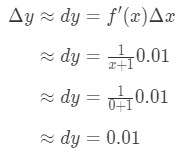
Equation 6: Differential question pt.3 Hence, y 0.01
However, most of the time we want to estimate a value of the function, and not the change of the value. Hence we will add both sides of the equation by y, which gives us:

which is the same as:

This equation is a bit hard to read, so we are going to rearrange it even more. Let's try to get rid of y and y. Notice that y+ y is basically the same as finding the value of the function at x+x. In other words,

Hence substituting this in our approximation above will give us:

where f(x+x) is value we are trying to estimate. How do we use this formula? I recommend following these steps:
- Step 1: Set the number equal to f(x+x). Find x, x, and f(x).
- Step 2: Calculate f'(x)
- Step 3: Use the formula to approximate the number
Let's use these steps for the following question.
Question 5: Use differentials to approximate .
- Step 1: Compare f(x+x) with . Since has a square root and 9 is a perfect square that is closest to 10, then let
Notice that:

Equation 7: Approximate value with differentials pt.1 See that there is no choice but to let x = 1
Equation 7: Approximate value with differentials pt.2 - Step 2:
See that the derivative gives:

Equation 7: Approximate value with differentials pt.3 So this implies
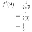
Equation 7: Approximate value with differentials pt.4 - Step 3:
Plugging everything into the formula gives us:
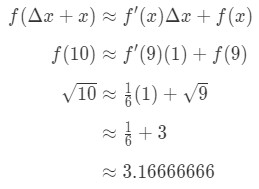
Equation 7: Approximate value with differentials pt.5 Hence, we just approximated the number.
One interesting thing to note is that linear approximation and differentials both give the same result for .
If you want to learn more about differentials, click this link:
http://tutorial.math.lamar.edu/Classes/CalcI/LinearApproximations.aspx
Proving L'Hospital's Rule using linear approximation
Now we have learned a lot about linear approximation, but what else can we do with it? We can actually use the linear approximation formula to prove a rule known as L'Hospital's Rule . Here is how the proof works.
Recall that the linear approximation formula is:

See that we can rearrange the formula so that:
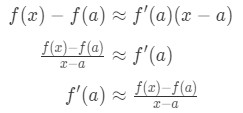
Realize that the approximation becomes more and more accurate as we pick x values that are closer to a. In other words if we take the limit as x→a, then they will equal. So

Now we are going to put this aside and use it later, and actually look at l'hopital's rule. We are going to assume a couple things here. Suppose that f(x) and g(x) are continuously differentiable at a real number a, f(a)=g(a)=0, and g'(a) 0. Then,
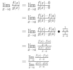
Now notice that we can apply the formula that we derived earlier right here. So now

Now instead of writing f'(a) and g'(a), we can apply limits as x→a (because we know f and g are differentiable). So

Hence, we just showed that:

which is L'Hospital's Rule .
When to use l'hopital's rule
We always want to apply l'hoptial's rule when we encounter indeterminate limits. There are two types of indeterminate forms. These indeterminate forms would be:

A lot of people make the mistake of using l'hopital's rule without even checking if it is an indeterminate limit. So make sure you check it first! Otherwise, it will not work and you will get the wrong answer. Here is a guide to using l'hopital's rule:
- Step 1: Evaluate the limit directly.
- Step 2: Check if it is one of the indeterminate forms. If it is, go to step 3.
- Step 3: Use l'hopital's rule.
- Step 4: Check if you get another indeterminate form. Repeat Step 3 if you do.
Let's take a look at a few examples using these steps.
Question 6: Evaluate the limit

- Step 1: Evaluating the limit directly gives us

Equation 9: L'hopital's rule question pt.2 - Step 2:
Yes, it is one of the indeterminate forms.
- Step 3:
Applying l'hopital's rule we have:
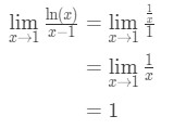
Equation 9: L'hopital's rule question pt.3 - Step 4:
one is not an indeterminate form, so we are done and the answer is 1.
Now that question was a little bit easy, so why don't we take a look at something that is a bit harder.
Question 7: Evaluate the limit

- Step 1: Evaluating the limit directly we see that:

Equation 10: L'hopital's rule twice question pt.2 - Step 2:
This is an indeterminate form, so go to step 3.
- Step 3:
Applying l'hopital's rule we have
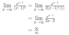
Equation 10: L'hopital's rule twice question pt.3 - Step 4:
This is another indeterminate form. So we have to go back to step 3 and apply l'hoptial's rules again.
- Step 3:
Applying l'hopital's rule again we have:

Equation 10: L'hopital's rule twice question pt.4 - Step 4:
Infinity is not an indeterminate form, so we are done and the answer is
Use a linear approximation to estimate a given number:
1) identify the corresponding function
2) pick an appropriate "a", such that:
-"a" is within a reasonable range
- is easy to evaluate
3) set up the linear approximation formula:
- for near a:
4) estimate the given number!


