Transform Linear Systems into Powerful Matrix Representations

Unlock the potential of linear systems by mastering matrix representation. Simplify complex equations, visualize relationships, and solve problems efficiently with this essential linear algebra skill.

Representing a linear system as a matrix

How to do matrices

Although the subtitle of this section may sound like a silly question since we already had a whole lesson on notation of matrices, this lesson will be completely about that: how to build matrices, specifically, how to write down matrices which represent and aid to solve the system of equations provided in certain problems.

From algebra we already know how to solve system of linear equations, and we know that in order to solve a certain system we require the same amount of unknowns (which we call variables) as the amount of equations in the system. We have studied methods on how to resolve them, such as the method of substitution, elimination and even in the past lesson we were solving systems of linear equations by graphing . Now is time to learn how to do it by knowing how to solve matrices.

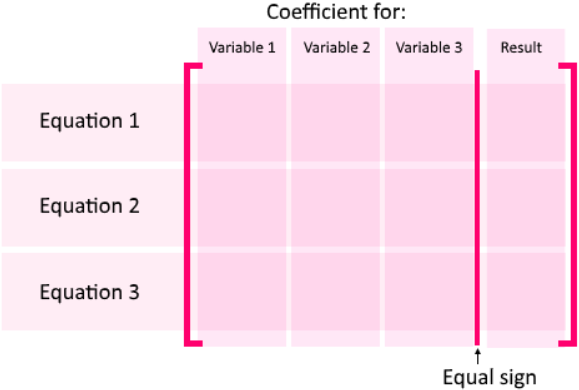
So let us construct the matrix in question then! For a linear system of three equations with three unknowns, the general diagram below works perfectly. We will be constructing a matrix such that all of the coefficients from the variables in each equation will be used as elements in the matrix. Notice the equations will be piled as the rows, and since we have three different variables, we start by putting the coefficient of each of them, for each equation in the order signaled in figure 1.


As a simple example, let us look at a three-equations-for-three-unknowns system and how this would be distributed when writing it as a matrix:


Notice that while passing the coefficients found in each equation as part of a linear system of equations, the type of coefficient in each case can make the matrix notation a little bit tricky, and for that, let us list a few important rules to remember while representing a linear system as a matrix:

• The signs of the coefficients must be carried to the matrix.


• If one of the terms in an equation from the system does not have a coefficient, it means the coefficient is a 1 and this will be the number which will be placed in its proper place on the matrix representation of the linear equations system.
• If there is not a numerical coefficient preceding a variable on an equation, but there is a negative sign, then the corresponding value to put on the matrix representation is -1.


• Always check the maximum amount of variables in the equations from the system, when passing them to matrix form, it is important that you have the same amount of unknowns as the same amount of equations, this means that you will have the same amount of rows and columns on the left hand side of the augmented matrix, which is the final matrix notation for the system.
• When one of the equations on the system has less terms than the rest (one or a few variables do not appear on this equation). The coefficient that will be placed on the matrix for this terms space will be a zero.


• The vertical line inside the matrix represents the equal sign, and so, all of the values in the right hand side from the equal sign on each equation, MUST be on the right hand side of the vertical line in the matrix.

Is worth noting that so far all we did was augmenting. In other words, to solve the system of equations in figure 2 there is much more than just transcribing the system into a different notation, such as compute elementary row operations, etc. That is not the topic of today, this lesson is not about how to solve the system, but just how to transform it into an augmented matrix.

What is an augmented matrix

What you saw in the right hand side of from figure 2 as the matrix representation of a linear system of equations is what we call an augmented matrix.


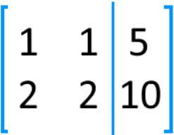
An augmented matrix will have as many columns to the left of the vertical line as there are possible variables from a system of equations. This means that on the left hand side of the augmented matrix from the vertical, you must have something like a square matrix (same amount of rows as columns). This particular characteristic must be met due to the fact that, as we have mentioned before, in algebra you need to have as many equations as unknowns in order to solve a system of equations and to secure to find the solution for all of the variables.

Therefore, in an augmented matrix you have each of your equations represented as rows, each column defines a variable and the digit on each element corresponds to the constant coefficient of the particular variable on the specific equation.

We can clearly observe this on figure 1. Notice that the system of equations contain three different variables: $x$, $y$ and $z$. And thus, even when some of the equations do not contain all of the possible variables, still their place is kept in the matrix representation and just filled up with a zero. This makes an augmented matrix a very orderly manner to represent a system of equations, it allows you to see side by side the comparison between the quantities of each type of variable among the equations in the system.

And what if your system of equations contains more than two or three variables and thus more than two or three equations? Easy! You can build an augmented matrix as big as necessary, just keep on adding columns to the left of the vertical line and of course rows to the whole matrix.


The augmented matrix method provides a simplistic method to solve system of equations in a more graphic, yet strictly algebraic manner. This method is a clean way to observe the quantity (coefficient) associated to each variable in an organized fashion that will allow spatial-oriented mathematicians to relate it to their quantities.

The augment definition gives us a better picture of the point above, augmenting means to expand, to add, to supplement. An augmented matrix is one which places two supplementing matrices together into one, side by side, in order for them to all be affected by a single operation computed on the matrix at the same time. Such operations applied to the augmented matrix are what we call row operations (or matrix row reduction) and is the equivalent to trying to solve system of linear equations through substitution.

In the algebraic method of substitution, we know the main rule says that whichever operation is done on the left hand side of an equation in the system, it must be performed too on its right hand side. Clearly said: whichever operation you apply to an equation must operate on all of the terms inside of such equation, in either side of its equal sign, in order to keep the proportionality relationship of the variables inside the equation.

Thus, and augmenting matrix and its methodology provide the perfect environment to keep this rule. The two matrices being put together here would be either side of the vertical line, and so, whichever operation done in one side of this vertical line is automatically done on the other side thus keeping the proportionality relationship of the variables in the system. Such operations will be seen in a later lesson on this Linear Algebra course.


Again, although this will be explained in much more detail on the lessons to follow, we will summarize in the next list, the steps followed when solving matrix equations. Thus, the next is the general process of solving system of equations by representing a linear system as a matrix:

1. Converting the system of equations into an augmented matrix
2. Perform matrix row operations following Gaussian elimination or Gaus Jordan elimination to obtain the matrix row echelon form or if needed its reduced row echelon form
3. Transcribe the simplified set of linear equations resulting from elimination:
1. If the previous elimination resulted in a matrix of row echelon a simplified system of equations may be transcribed from it where most of the variables have been solved.
2. If the previous elimination resulted in a matrix of reduced row echelon form a system of equations, which has been simplified to the maximum, may be obtained from such matrix. In which case most if not all of the variables would have been solved.
1. In such cases, the general solution of the augmented matrix has been found.
4. If the system of simplified equations does not shows the explicit solutions of all variables, solve for the ones left through basic algebra substitution.

As you can see, there are many new terms we need to learn first before we can solve a system of equations through matrices math. Whole lessons on the three types of matrix row operations, row reduction and echelon forms are needed for you to have the complete picture about solving a linear system with matrices using Gaussian elimination. On this lesson, we focus on just the change of notation from basic algebraic expressions to a matrix equation to have a solid base by the time we can compute solution sets of linear systems in their totality.
If you want to continue your studies on how to represent linear systems with matrices equations we recommend you to take a look into this link.

And so, to finish this lesson, let us work through a few simple examples of what this lesson was about: To define augmented matrices for linear systems of equations.

Write the augmented matrix for each system of equations

For the next exercises we will be writing the matrix equation which correctly represents the system of equations in the left. Some systems may be a little bit more complicated or tricky than others, but notice how all of them follow the process described in figure 1. Try to work them all on your own following the instructions given with figure 1 and the set of steps in the first section of this lesson, if you have problems with any of them go back and check the videos of this lesson, which include extended explanations of each case.

Example 1

Represent the next system of linear equations as a matrix:

$\large x + 6y - 3z = 3$
$4x + 2y - z = 10$
$6x + 10y + 20 z = 0$
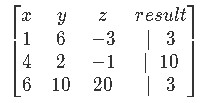
This system has three different variables: $x$, $y$ and $z$. And it has three equations, thus, the resulting augmented matrix must have three columns on its left side and consist of three rows:

$\large x + 6y - 3z = 3$
$4x + 2y - z = 10$
$6x + 10y + 20 z = 0$
$\downarrow$

Example 2

Represent the next system of linear equations as a matrix:

$\large -3x + 7y = 10$
$10x + 2y = 15$
For this case we have a system with two equations for two unknowns, thus two rows and two columns on the left side of the vertical line in the augmented matrix.

$\large -3x + 7y = 10$
$10x + 2y = 15$
$\Downarrow$

Example 3

Represent the next system of linear equations as a matrix:

$\large v + w + x + y + z = 0$
$x + y + z = 5$
$x + y = 3$
$2v + 4w = 2$
$y = 3$
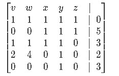
On this system we have five unknowns (variables) thus we must have five columns on the left side of the augmented matrix. Notice that one variable is already solved for us in the last equation, but at this moment do not worry about that since we are only caring about transforming the system into the matrix. Five equations means five rows and remember that for any equation not containing certain variables, it means you have to put a zero in the place of their coefficients in the matrix. Thus the matrix looks as follows:

$\large v + w + x + y + z = 0$
$x + y + z = 5$
$x + y = 3$
$2v + 4w = 2$
$y = 3$
$\Downarrow$

Example 4

Represent the next system of linear equations as a matrix

$\large 9x = 3$
This particular system can look as if extremely tricky, in reality is as simple as it looks: one equation for one unknown: one row in the augmented matrix and one column (in this case just one element) on its left side.

$\large 9x = 3$
$\Downarrow$

Example 5

Represent the next system of linear equations as a matrix:

$\large 2w + 6y + 2z = 3$
$3x + 6y = 2$
$x + y + z = 10$
$w + 2x +10y + z = 7$
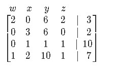
Something important to remember here is that before to get a preconceived image of your augmented matrix in your head, always make sure to check all of the equations contained in the system. For this particular system notice how we could be biased to believe we only have three variables to accommodate, when it is seen until the very last equation that we actually have four variables.

It is true that you may just look into the number of equations you have in a system and automatically just think to make the left hand side of the augmented matrix you are about to construct similar to a square-like matrix, the issue is, although we need a system of the same number of equations as unknowns (variables) to find the explicit solution of a system, that is NOT to say you cannot construct an augmented matrix with a system containing any different amount of equations and its variables. Actually, you can do an augmented matrix with any amount combination of these two things (it doesnt matter how many equations and variables are in the system) just the way how to solve them and its possibility changes, but the notation transformation can be done nonetheless.

You will observe this in examples 7, 8 and 9 below. Now let us construct the matrix for equation 10:

$\large 2w + 6y + 2z = 3$
$3x + 6y = 2$
$x + y + z = 10$
$w + 2x +10y + z = 7$
$\Downarrow$
Now to finalize our lesson we will work on some example exercises which require us to now go the other way around, from matrix equation notation to write down the linear system of equations in regular algebraic expressions: